
Early Childhood
Greater Louisville Project
2021
Data used in this report is reflective of pre-COVID trends throughout our community. The effects of COVID on child development and kindergarten readiness are not yet fully known or understood, but as the report below will show children not participating in a formal setting before kindergarten have the lowest kindergarten readiness scores. In 2020, child care providers were mandated to close from March 20 to June 15th due to COVID and operated at reduced capacity until March 15, 2021. In addition, many providers have closed permanently, or had to close on and off as a result of COVID cases at their site. Due to these realities we know that more children than ever will have spent the last year at home and not in a formal care setting.
Introduction
The first five years of a child’s life provide the building blocks for lifelong learning and health. While Louisville has a large ecosystem of individuals, businesses, and organizations that support early childhood development, many families across Louisville face barriers to accessing those resources.
This report analyzes one way to evaluate early childhood development—kindergarten readiness—as well as several factors that impact it: the price and availability of child care, adverse childhood experiences, and food security. We chose these data based on community interest and with the aim of illuminating topics for which local data is not widely available.
Wherever possible, we analyze the connection between race, geography, and early childhood development. As a result of institutional racism, residential segregation, discriminatory policies, and many other factors, Louisville’s early childhood system does not support all populations equally. In support of A Path Forward, we focus on Black children in particular. However, structural racism does not just affect Black children, and exclusionary policies affect people based on more identities than their race and ethnicity. While we provide some data that extends beyond race, data for other races and populations in our community is often limited, a problem in its own right.
The Greater Louisville Project created this report in conjunction with the Louisville Urban League, which has recently convened community members around A Path Forward and has assisted African Americans and other marginalized populations in attaining social and economic equality in Louisville for over 100 years. This report was also produced in conjunction with the Ready for K Alliance, whose vision is that all children enter kindergarten ready to thrive.

![]()
Join experts for an open community conversation about early childhood on May 18, 2021. Register for this free, virtual event here.
Kindergarten Readiness
Kindergarten readiness is an important indicator of whether children will succeed in the classroom for years to come. Based on data from KySTATS, JCPS students who entered school ready for kindergarten in 2016 were over three times as likely to achieve test results at or above their grade level on their standardized K-PREP math and reading tests in the 3rd grade. This is true for both JCPS students as a whole and Black JCPS students in particular.
Kentucky school districts evaluate kindergarten readiness using the BRIGANCE Early Childhood Kindergarten Screen III, which assesses child development across five areas:
- Academic/Cognitive Development
- Language Development
- Physical Development
- Self-Help Skills
- Social and Emotional Skills
The BRIGANCE screener asks children to perform tasks such as identifying letters, numbers, and shapes or using a writing utensil. Parents and caregivers provide information on their child’s self-help, social, and emotional skills such as whether their child can dress themselves, communicate their feelings, or take turns with other children. The results of this screening are a strong indicator of a student’s future academic performance.
It is important to note that the BRIGANCE screener has limitations. For example, children enrolled in child care are more likely to receive instruction tailored to the BRIGRANCE screener than children in a home setting with their parents or a caregiver. While many of the topics and questions represent important developmental foundations, child development includes factors beyond just the questions in BRIGANCE. It is important to consider how results are affected by cultural bias in all tests and screeners, including BRIGANCE. Communicating the developmental milestones in BRIGANCE to all families can ensure that kindergarten readiness truly measures healthy development and not just preparation for the screener.
Examples of questions included in BRIGANCE can be viewed here:
- Example child assessment (academic, language, and physical measures)
- Example parent report (self-help, social, and emotional skills)
Kindergarten readiness data was acquired through the Kentucky Department of Education and through data requests to JCPS. The data only include students who enter JCPS, so students who attend private school or who are homeschooled are not included in the data. To view more data on kindergarten readiness, you can visit our Kindergarten Readiness page.
Overall Readiness
Since JCPS began tracking kindergarten readiness in 2012-13, overall readiness levels have fluctuated up to five percentage points per year but have remained largely unchanged. Other Kentucky students have seen their scores slightly increase, but overall JCPS readiness levels are higher than the state average.
load("raw_data/kready_ky.RData")

kready_ky %<>%
  mutate(year = year - 1)

kready_total <- kready_ky %>%
  filter(sex == "total",
         race == "total",
         frl_status == "total",
         prior_setting == "All Students") %>%
  filter(variable %in% c("lou", "mean")) %>%
  mutate(District = if_else(variable == "lou", "JCPS", "Other Kentucky Districts"))

plt_by(kready_total,
       District,
       kready,
       title_text = "Kindergarten Readiness",
       caption_text = "Source: Greater Louisville Project
                       Data from the Kentucky Department of Education School Report Card",
       school = T,
       y_min = 40,
       ymax = 60)
By Race
Racial disparities in kindergarten readiness have been largely persistent since the 2012-13 school year. The kindergarten readiness gap between Black students and white students shrank from 12 points in 2012-13 to around 5 points in 2016-17 before growing again. As of the 2018-19 school year, scores for the four groups included here are all within five points of their original levels, but vary by up to 30 percentage points between student groups.
kready_race <- kready_ky %>%
  filter(variable == "lou",
         sex == "total",
         race %in% c("black", "white", "hispanic", "asian"),
         frl_status == "total",
         prior_setting == "All Students") %>%
  mutate(Race = str_to_title(race))

plt_by(kready_race,
       Race,
       kready,
       school = T,
       title_text = "JCPS Kindergarten Readiness by Race",
       caption_text = "Source: Greater Louisville Project
                       Data from the Kentucky Department of Education School Report Card",)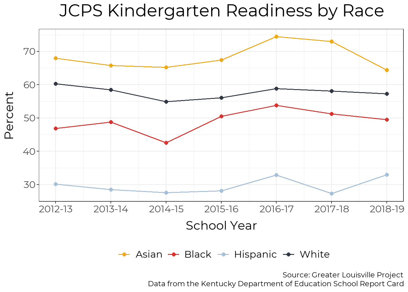
By Prior Setting
The largest differences in kindergarten readiness among student groups are based on prior setting.
Children who were enrolled in child care, as reported by their parent or caregiver, prior to entering school are most likely to be kindergarten ready, while children who stayed at home with a parent or caregiver are least likely to be kindergarten ready.
Children whose prior setting was Head Start, a state-funded preschool program, or were in another home setting such as a private sitter or other family member (labeled “Other”), fall in the middle.
Public (state-funded) preschool is available to 4-year-olds who live in a household with an income up to 160% of the federal poverty level and to 3- and 4-year-olds with disabilities. Head Start is available to children age birth to 5 who live in a household with income up to 100% of the federal poverty level. You can find the current federal povery levels here.
kready_louisville <- kready_ky %>%
  filter(variable == "lou",
         sex == "total",
         race == "total",
         frl_status == "total",
         prior_setting %in% c("State Funded", "Head Start", "Child Care", "Home", "Other")) %>%
  mutate(prior_setting = if_else(prior_setting == " State Funded", "State-Funded", prior_setting))

kready_louisville2 <- kready_ky %>%
  filter(variable == "lou",
         sex == "total",
         race %in% c("black", "total"),
         frl_status == "total",
         prior_setting %in% c("State Funded", "Head Start", "Child Care", "Home", "Other")) %>%
  mutate(prior_setting = if_else(prior_setting == " State Funded", "State-Funded", prior_setting))

plt_by(kready_louisville,
       prior_setting,
       kready,
       school = T,
       title_scale = 0.95,
       title_text = "JCPS Kindergarten Readiness by Prior Setting",
       caption_text = "Source: Greater Louisville Project
                       Data from the Kentucky Department of Education School Report Card",
       remove_legend_title = T)
Prior Setting by Race
The graph below shows the prior setting of students entering JCPS kindergarten in 2019. About 60% of students were enrolled in child care or preschool outside the home, and around 40% of students were at home with their parents or another caregiver.
Students who are white, Asian, American Indian or Alaska Native, or of two or more races are more likely than average to be enrolled in child care outside of the home before entering JCPS. Students who are Black are much less likely to be enrolled in child care, but much more likely to be enrolled in state-funded preschool. Hispanic students and students whose race is not known are much more likely to be in a home setting.
prior_setting_race <- readxl::read_excel("raw_data/ORR DRMS 9969 MetroUnitedWay.xlsx",
                                         sheet = "Race", skip = 1)

prior_setting_race %<>%
  pivot_longer(cols = `State Funded`:Other, names_to = "Prior Setting", values_to = "count") %>%
  filter(!is.na(count)) %>%
  group_by(Race) %>%
  mutate(
    percent = count / sum(count) * 100,
    count = scales::comma(count, accuracy = 1)) %>%
  ungroup() %>%
  mutate(
    Race = if_else(Race == "Grand Total", "All JCPS Students", Race),
    Race = if_else(Race == "White (Non-Hispanic)", "White", Race),
    Race = if_else(Race == "African American", "Black", Race),
    Race = if_else(Race == "American Indian or Alaska Native", "American Indian or<br>Alaska Native", Race),
    Race = factor(Race, levels = rev(c("All JCPS Students",
                                   "American Indian or<br>Alaska Native",
                                   "Asian",
                                   "Black",
                                   "Hispanic",
                                   "White",
                                   "Two or more races",
                                   "Unknown")),
                  ordered = TRUE),
    `Prior Setting` = if_else(`Prior Setting` == "State Funded", "State-Funded", `Prior Setting`),
    `Prior Setting` = factor(`Prior Setting`,
                             levels = rev(c("Child Care", "State-Funded", "Head Start",
                                        "Other", "Home")),
                             ordered = TRUE))

plot_ly(prior_setting_race,
        x = ~percent, y = ~Race,
        color = ~`Prior Setting`,
        colors = c("Child Care" = "#d63631",
                   "State-Funded" = "#323844",
                   "Head Start" = "#eaab21",
                   "Other" = "#a7bfd7",
                   "Home" = "#7CE3B6"),
        text = ~`count`,
        type = 'bar',
        hovertemplate = paste('Percent: %{x:.1f}%<br>Number: %{text}<extra></extra>')) %>%
  layout(
    title = "JCPS Prior Setting by Race",
    font = list(family = "Montserrat"),
    barmode = 'stack',
    yaxis = list(title = ""),
    xaxis = list(title = "Percent"),
    legend = list(title = list(text = "Prior Setting")))
Prior Setting by Zip Code
Among children who enter JCPS, children in the Highlands and in Eastern Louisville are more likely than average to be enrolled in child care before entering JCPS. Children in West Louisville are most likely to be enrolled in state-funded preschool at JCPS, and children in South Louisville are most likely to be in a home setting.
prior_setting_zip <- readxl::read_excel("raw_data/ORR DRMS 9969 MetroUnitedWay.xlsx",
                                        sheet = "Zip Code", skip=1)

prior_setting_zip %<>%
  mutate(
    zip = `Zip Code`,
    total_students = `State Funded` + `Head Start` + `Child Care` + Home + Other) %>%
  mutate(across(`State Funded`:`Other`, ~ . / total_students * 100)) %>%
  filter(!is.na(zip))

prior_setting_map <- map_zip %>%
  left_join(prior_setting_zip, by = "zip")

pal <- colorNumeric("viridis", domain = c(0, 75))

m <- leaflet(prior_setting_map) %>%
  addTiles() %>%
  addPolygons(
    color = "#444444", fillOpacity = 0.9, weight = 2, smoothFactor = 0.5,
    fillColor = ~pal(`Child Care`), group = "Child Care") %>%
  addPolygons(
    color = "#444444", fillOpacity = 0.9, weight = 2, smoothFactor = 0.5,
    fillColor = ~pal(`State Funded`), group = "State-Funded") %>%
  addPolygons(
    color = "#444444", fillOpacity = 0.9, weight = 2, smoothFactor = 0.5,
    fillColor = ~pal(`Head Start`), group = "Head Start") %>%
  addPolygons(
    color = "#444444", fillOpacity = 0.9, weight = 2, smoothFactor = 0.5,
    fillColor = ~pal(`Home`), group = "Home") %>%
  addPolygons(
    color = "#444444", fillOpacity = 0.9, weight = 2, smoothFactor = 0.5,
    fillColor = ~pal(`Other`), group = "Other") %>%
 addLegend(pal = pal, values = c(0, 75), opacity = 0.7,
           title = "Percent") %>%
 addLayersControl(baseGroups = c("Child Care", "State-Funded", "Head Start", "Home", "Other"),
                  options = layersControlOptions(collapsed = F))

css_fix <- ".leaflet .leaflet-control {font-family: Montserrat;}"
html_fix <- htmltools::tags$style(type = "text/css", css_fix)
m %<>% htmlwidgets::prependContent(html_fix)

htmlwidgets::saveWidget(m, file = "index_maps/prior_setting_zip.html")
knitr::include_url("index_maps/prior_setting_zip.html")
By Race and Prior setting
Combining the analysis by race and prior setting shows which settings are most effective at ensuring children enter kindergarten ready to thrive. Click on the dropdown box on the right of the graph to view the data for each prior setting.
Among the groups we examine here, the smallest racial disparities exist among children who were previously enrolled in Head Start or state-funded preschool. This is likely due to the fact that families must meet certain income limits to enroll their children in these programs, so children in these programs come from families with common economic situations. Black and Brown children in these settings enter kindergarten with relatively high readiness rates, and they have seen improvements since 2013-14.
Students enrolled in child care settings have the highest kindergarten readiness rates, however, racial disparities for these children are wider than for all children. As will be discussed later, this reflects differences in access to affordable and high-quality child care.
Differences in kindergarten readiness among children who were previously in a home setting with their parents or caregivers (Home) or in another home-based setting (Other) are difficult to interpret because it reflects a wide variety of experiences for children. On average, children who were previously at home with their parents or caregvers enter kindergarten the least ready to learn.
kready_race_plotly <- kready_ky %>%
  filter(variable == "lou",
         sex == "total",
         race %in% c("black", "white", "hispanic", "asian"),
         frl_status == "total",
         prior_setting %in% c("All Students", "State Funded", "Head Start", "Child Care", "Home", "Other")) %>%
  mutate(
    race = str_to_title(race),
    prior_setting = if_else(prior_setting == "State Funded", "State-Funded", prior_setting)) %>%
  pivot_wider(names_from = race, values_from = kready) %>%
  mutate(year_label = paste0(year - 1, "-", year - 2000))

trnfm_list <-
  list(
      list(
        type = 'filter',
        target = ~prior_setting,
        operation = 'in',
        value = unique(kready_race_plotly$prior_setting)[1]))

plot_ly(kready_race_plotly, width = "100%") %>%
  add_trace(x = ~year_label, y = ~Asian, name = "Asian", type = "scatter", mode = "lines",
            line = list(color = '#a7bfd7', width = 2),
            marker = list(color = '#a7bfd7', size = 6),
            transforms = trnfm_list) %>%
  add_trace(x = ~year_label, y = ~Black, name = "Black", type = "scatter", mode = "lines",
            line = list(color = '#d63631', width = 2),
            marker = list(color = '#d63631', size = 6),
            transforms = trnfm_list) %>%
  add_trace(x = ~year_label, y = ~Hispanic, name = "Hispanic", type = "scatter", mode = "lines",
            line = list(color = '#eaab21', width = 2),
            marker = list(color = '#eaab21', size = 6),
            transforms = trnfm_list) %>%
  add_trace(x = ~year_label, y = ~White, name = "White", type = "scatter", mode = "lines",
            line = list(color = '#323844', width = 2),
            marker = list(color = '#323844', size = 6),
            transforms = trnfm_list) %>%
  layout(title = "JCPS Kindergerten Readiness by Race",
         font = list(family = "Montserrat"),
         xaxis = list(title = "Year"),
         yaxis = list(title = "Percent Ready", range = c(0, 100)),
         hovermode = "x unified",
         updatemenus = list(
          list(
            x = 1.25,
            y = 0.75,
            buttons = list(
              list(method = "restyle",
                   args = list("transforms[0].value", unique(kready_race_plotly$prior_setting)[1]),
                   label = unique(kready_race_plotly$prior_setting)[1]),
              list(method = "restyle",
                  args = list("transforms[0].value", unique(kready_race_plotly$prior_setting)[2]),
                  label = unique(kready_race_plotly$prior_setting)[2]),
              list(method = "restyle",
                  args = list("transforms[0].value", unique(kready_race_plotly$prior_setting)[3]),
                  label = unique(kready_race_plotly$prior_setting)[3]),
              list(method = "restyle",
                  args = list("transforms[0].value", unique(kready_race_plotly$prior_setting)[4]),
                  label = unique(kready_race_plotly$prior_setting)[4]),
              list(method = "restyle",
                  args = list("transforms[0].value", unique(kready_race_plotly$prior_setting)[5]),
                  label = unique(kready_race_plotly$prior_setting)[5]),
                            list(method = "restyle",
                   args = list("transforms[0].value", unique(kready_race_plotly$prior_setting)[6]),
                   label = unique(kready_race_plotly$prior_setting)[6])))))
By Geography
Student Zip Code
The data show wide disparities in kindergarten readiness across Louisville. Because some zip codes contain small numbers of students, we combine data over three years to increase the reliability of the data. Kindergarten readiness by zip code ranges from 30% in 40118 to 81% in 40205.
# Kready math

# ready w/ enrichments * (% distinguished + % proficient)
ready_prof_dist_math = (643 * (.317 + .353) + 2956 * (.122 + .355)) /
                    (643 * (1 - .143) + 2956 * (1 - .111)) * 100
not_ready_prof_dist_math = 3886 * (.034 + .160) / 3886 * (1 - .111) * 100

mult_math = ready_prof_dist_math / not_ready_prof_dist_math

# Kready reading
ready_prof_dist_reading = (643 * (.463 + .235) + 2956 * (.219 + .309)) /
                    (643 * (1 - .143) + 2956 * (1 - .111)) * 100
not_ready_prof_dist_reading = 3886 * (.057 + .165) / 3886 * (1 - .111) * 100

mult_reading = ready_prof_dist_reading / not_ready_prof_dist_reading

# black children
# ready w/ enrichments * (% distinguished + % proficient)
ready_prof_dist_math = (149 * (.148 + .376) + 940 * (.044 + .234)) /
                    (149 * (1 - .067) + 940 * (1 - .089)) * 100
not_ready_prof_dist_math = 1443 * (.013 + .089) / 1443 * (1 - .090) * 100

mult_math_black = ready_prof_dist_math / not_ready_prof_dist_math

# Kready reading
ready_prof_dist_reading = (149 * (.275 + .248) + 940 * (.091 + .240)) /
                    (149 * (1 - .067) + 940 * (1 - .089)) * 100
not_ready_prof_dist_reading = 1443 * (.019 + .106) / 1443 * (1 - .090) * 100

mult_reading_black = ready_prof_dist_reading / not_ready_prof_dist_reading

race_math = mult_math_black / mult_math
race_reading = mult_reading_black / mult_reading


# Ready in kready data
kready_zip <- readxl::read_excel("raw_data/Copy of 1920_Brigance Zip Code_Prior Settings TablesForORR.xlsx",
                                 sheet = "ZipCode3Years",
                                 range ="B4:K38",
                                 col_names = c("zip", paste0(c("num_", "ready_", "notready_"),
                                                             rep(2018:2020, each = 3))),
                                 col_types = c("text", rep("numeric", 9)),
                                 na = "*")

# Clean and organize data frame
kready_zip %<>%
  pivot_longer(num_2018:notready_2020, names_to = c("var_type", "year"), names_sep = "_") %>%
  filter(var_type != "notready") %>%
  mutate(
    var_type = case_when(var_type == "num" ~ "population",
                         var_type == "ready" ~ "percent")) %>%
  transmute(
    zip, year, var_type,
    kready = if_else(var_type == "percent", value * 100, value))

# Summarize data frame over three years due to unstable data
kready_zip_sum <- kready_zip %>%
  pivot_wider(names_from = var_type, values_from = kready) %>%
  group_by(zip) %>%
  filter(all(!is.na(percent))) %>%
  summarise(
    percent = weighted.mean(percent, population),
    population = sum(population),
    .groups = "drop") %>%
  rename(kready = percent)

# Join data to map
map_zip %<>% left_join(kready_zip_sum, by = "zip")

ggplot(map_zip) +
  geom_sf(aes(fill = kready), color = "white") +
  #scale_fill_manual(values = viridis::viridis(6, direction = -1), na.value = "grey") +
  viridis::scale_fill_viridis(na.value = "grey",
                            name = "Percent Ready") +
  theme_bw(base_size = 22, base_family = "Montserrat") +
  theme(panel.grid = element_blank(),
        axis.text = element_blank(),
        axis.ticks = element_blank(),
        axis.title = element_blank(),
        panel.border = element_blank()) +
  labs(title = "JCPS Kindergarden Readiness by Student's Home Zip Code",
       subtitle = "Average for the school years 2017-2018, 2018-2019, and 2019-2020",
       caption_text = "Source: Greater Louisville Project
                       Data from JCPS") +
  theme(plot.caption = element_text(lineheight = .5)) +
  theme(
    panel.background = element_rect(fill = "transparent", color = NA), # bg of the panel
    plot.background = element_rect(fill = "transparent", color = NA), # bg of the plot
    legend.background = element_rect(fill = "transparent", color = "transparent"), # get rid of legend bg
    legend.box.background = element_rect(fill = "transparent", color = "transparent"), # get rid of legend panel bg
    legend.key = element_rect(fill = "transparent",colour = NA))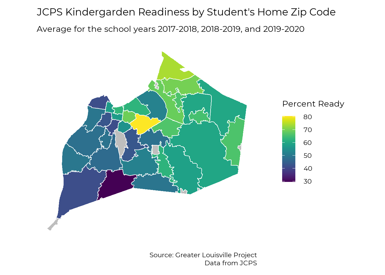
Elementary School
This map shows kindergarten readiness results by school. The areas on the map represent student assignment areas for individual schools. Kindergarten readiness by school varies from 13% to 89%.
load("raw_data/kready_jc.RData")
load("raw_data/map_elementary.RData")

# Filter out
kready_jc_subset <- kready_jc %>%
  filter(code != "275",
         year == 2020,
         demographic == "All Students",
         prior_setting == "All Students") %>%
  mutate(code = str_sub(code, 4, 6) %>%
                as.numeric)

map_elementary %<>%
  rename(
    SCHOOL_NAME = SCHOOL_NAM,
    LOCATION = LocNumber,
    CLUSTER = ClusterNum)

map_elementary %<>%
  left_join(kready_jc_subset, by = c("LOCATION" = "code"))

map_cluster <- map_elementary %>%
  group_by(CLUSTER) %>%
  summarise(
    kready = weighted.mean(kready, num_students),
    .groups = "drop")

ggplot(map_elementary) +
  geom_sf(aes(fill = kready), color = "white") +
  #scale_fill_manual(values = viridis::viridis(6, direction = -1), na.value = "grey") +
  viridis::scale_fill_viridis(na.value = "grey",
                            name = "Percent Ready") +
  theme_bw(base_size = 22, base_family = "Montserrat") +
  theme(panel.grid = element_blank(),
        axis.text = element_blank(),
        axis.ticks = element_blank(),
        axis.title = element_blank(),
        panel.border = element_blank()) +
  labs(title = "JCPS Kindergarden Readiness by School Location, 2019-2020",
       caption_text = "Source: Greater Louisville Project
                       Data from the Kentucky Department of Education School Report Card") +
  theme(plot.caption = element_text(lineheight = .5)) +
  theme(
    panel.background = element_rect(fill = "transparent", color = NA), # bg of the panel
    plot.background = element_rect(fill = "transparent", color = NA), # bg of the plot
    legend.background = element_rect(fill = "transparent", color = "transparent"), # get rid of legend bg
    legend.box.background = element_rect(fill = "transparent", color = "transparent"), # get rid of legend panel bg
legend.key = element_rect(fill = "transparent",colour = NA)) 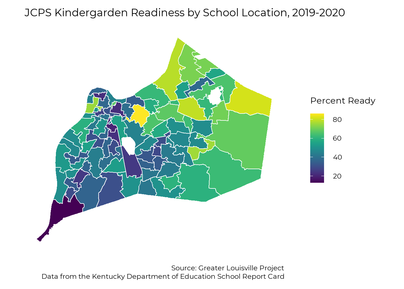
#geom_sf(data = map_cluster, fill=NA, color = "white", size = 1)Elementary School Cluster
This map shows kindergarten readiness results by elementary school clusters. Kindergarten readiness within school clusters varies from 31% to 68%.
ggplot(map_cluster) +
  geom_sf(aes(fill = kready), color = "white") +
  #scale_fill_manual(values = viridis::viridis(6, direction = -1), na.value = "grey") +
  viridis::scale_fill_viridis(na.value = "grey",
                            name = "Percent Ready") +
  theme_bw(base_size = 22, base_family = "Montserrat") +
  theme(panel.grid = element_blank(),
        axis.text = element_blank(),
        axis.ticks = element_blank(),
        axis.title = element_blank(),
        panel.border = element_blank()) +
  labs(title = "JCPS Kindergarden Readiness by School Cluster, 2019-2020",
       caption_text = "Source: Greater Louisville Project
                       Data from the Kentucky Department of Education School Report Card") +
  theme(plot.caption = element_text(lineheight = .5)) +
  theme(
    panel.background = element_rect(fill = "transparent", color = NA), # bg of the panel
    plot.background = element_rect(fill = "transparent", color = NA), # bg of the plot
    legend.background = element_rect(fill = "transparent", color = "transparent"), # get rid of legend bg
    legend.box.background = element_rect(fill = "transparent", color = "transparent"), # get rid of legend panel bg
    legend.key = element_rect(fill = "transparent",colour = NA))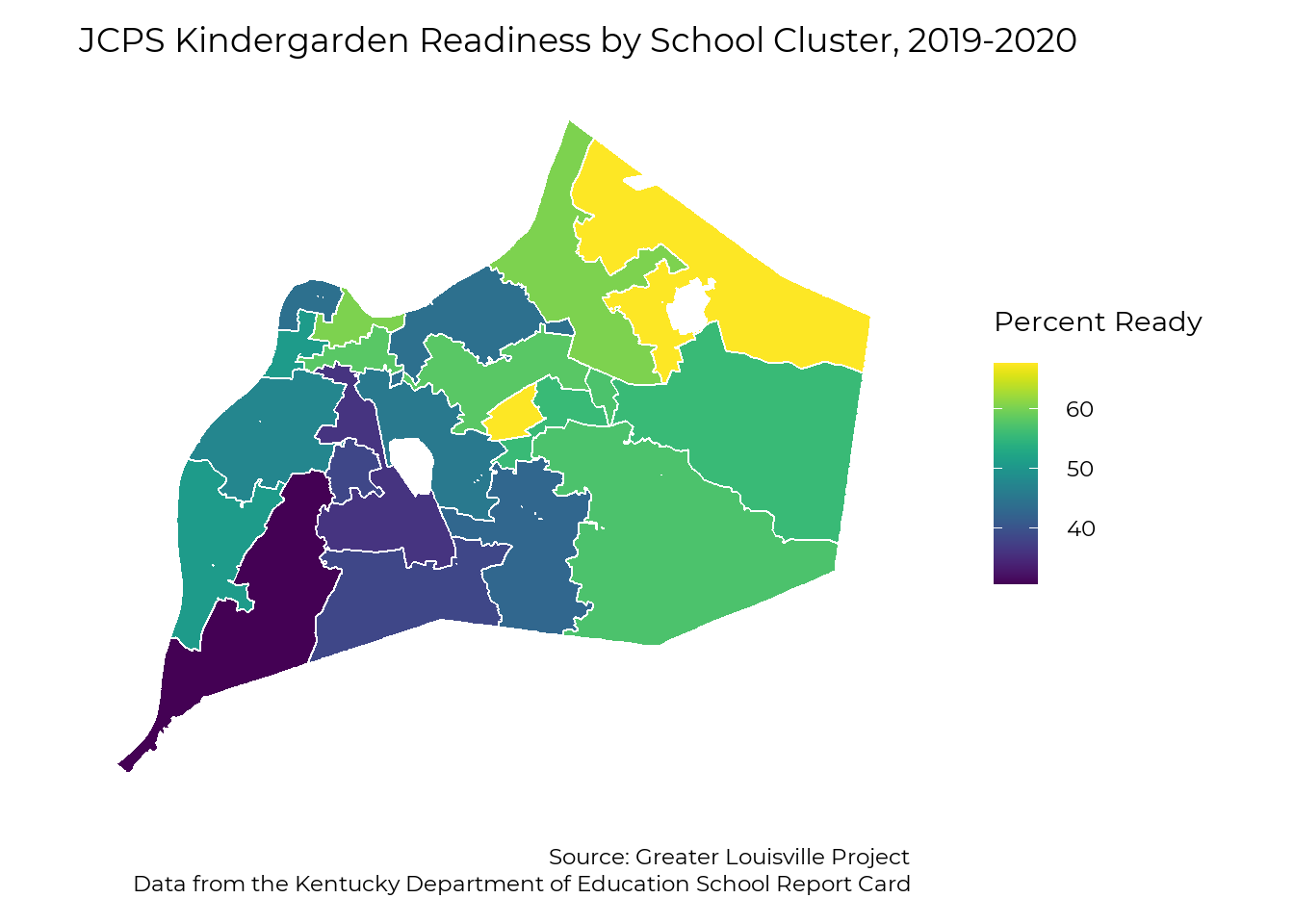
Early Child Care
High quality, affordable, and accessible child care is important for our community. As discussed in the prior setting section above, children in a child care setting enter kindergarten with the highest levels of kindergarten readiness. Additionally, reliable child care is important to ensure that parents and caregivers are able to work. However, child care is not affordable or accessible for many families.
Using data from kynect, we examine the price and availability of child care using information from child care providers. While providers should update their information anytime it changes, some data is not current, and many child care providers are in flux due to COVID-19. However, the kynect database is linked to the state registration system, and it is the most comprehensive source available at this time.
While our data examines the total licensed capacity of child care providers, the number of available child care slots is smaller. Licensed capacity is based solely on square footage, so many providers choose to serve a smaller actual capacity to maintain higher quality standards, due to issues retaining staff, or due to temporary barriers due to COVID-19.
Price
The median price of child care for one toddler is $8,710 per year, approximately 15% of the median household income for Jefferson County and 22% of the median household income for Black households in Jefferson County for 2019. We report daily rates in the charts below because that is the format provided by kynect. The median annual rate of $8,710 corresponds to a daily rate of $33.50.
Summary and Comparison to CCAP
The chart below shows the price of child care by age group and provider type compared to the maximum reimbursement rates for the Kentucky’s Child Care Assistance Program (CCAP). The column “Percent of Slots under CCAP” shows the percent of slots that would be fully paid for by CCAP.
# Creates four data frames linked by license number (CLR)

# provider_information: original file from the state.
#    includes provider name, address, and several other fields.

# provider_hours: includes open days and hours

# provider_cost: includes program offerings and cost

# provider_service_offerings: includes which age ranges are available

# provider_other: includes other available info.
#    Might just duplicate fields from program_information, though.

# Infant: <12 months
# Toddler: between 12 and 24 months
# School-age: child enrolled in kindergarten, elementary, or secondary education

# Read in provider information (county, name, address, etc.)
provider_information <- readxl::read_xlsx("raw_data/Chilcare Provider Download.xlsx",
                                          skip = 2)

# Subset to Jefferson County and rename license column for ease of use

provider_information %<>%
  filter(County == "JEFFERSON") %>%
  rename(CLR = `CLR#`) %>%
  filter(CLR != "C6739") %>%
  transmute(
    CLR,
    Name,
    Location = `Location Address`,
    Capacity,
    Transportation = if_else(`Transportation Service` == "Y", T, F),
    STARS = as.numeric(`Stars Rating`),
    Type = `Provider Type`,
    active_CCAP = if_else(`Active CCAP Children` == "Y", T, F),
    special_needs = case_when(
      `Serves Children with Special Needs` == "Y" ~ T,
      `Serves Children with Special Needs` == "N" ~ F,
      TRUE ~ NA),

    offerring = recode(`Age Range Of Service`,
                      "Infant" = 1,
                      "Infant To School Age" = 2,
                      "Infant To Two_To_School" = 3,
                      "Toddler To Two_To_School" = 4,
                      "Toddler To School_Age" = 5,
                      "Two_To_School" = 6,
                      "Two_To_School To School_Age" = 7,
                      "School_Age" = 8,
                      "No Information Available" = 9),

    Infant    = if_else(offerring %in% 1:3, T, F),
    Toddler   = if_else(offerring %in% 2:5, T, F),
    Preschool = if_else(offerring %in% 2:7, T, F),
    School    = if_else(offerring %in% c(2, 5, 7, 8), T, F)) %>%
  mutate(across(Infant:School, ~ if_else(offerring == 9, NA, .))) %>%
  select(-offerring)

# Read in provider data collected from KYnect
provider_data <- read_csv("raw_data/Childcare Provider Cost Data.csv",
                          col_names = c("CLR", "Day", "Time", "Services", "FullTime", "PartTime", "Other"))

# Check that no data is missing a license number - PASSED
# missing_CLR <- provider_data %>%
#   filter(is.na(CLR)) %>%
#   filter(!is.na(Day) | !is.na(Time) | !is.na(Services) |
#            !is.na(FullTime) | !is.na(PartTime) | !is.na(Other))
#
# # Check that the list of license numbers are identical - PASSED
# check_data1 <- mean(provider_information$CLR %in% provider_data$CLR) +
#                mean(provider_data$CLR %in% provider_information$CLR)

# Check values and number of each variable
# table(provider_data$Day) # good, 1 provider removed from listing
# table(provider_data$Time) # good
# table(provider_data$Services) # good
# table(provider_data$FullTime) # good
# table(test$PartTime) # often contains data for "Other"
# table(provider_data$Other) # good
# table(str_remove(provider_data$Other, "\\d*")) # good

# Filter out rows without license numbers (used to make data entry easier)
# Remove C6739, which closed between the creation of the provider registry and data collection
# Remove L355501, which is actually in Goshen
provider_data %<>%
  filter(!is.na(CLR),
         CLR %not_in% c("C6739", "L355501"))

# The data for the "Other" column is often located in the PartTime column.
# Group by license and determine whether the number of children is in the PartTime column. (should be in Other)
# If so, move the data from the PartTime column to the Other column for that provider.
provider_data %<>%
  group_by(CLR) %>%
  mutate(move_PartTime = if_else(any(str_detect(PartTime, "Children")), T, F),
         move_PartTime = if_else(is.na(move_PartTime), F, move_PartTime)) %>%
  mutate(Other = if_else(move_PartTime, PartTime, Other),
         PartTime = if_else(move_PartTime, NA_character_, PartTime)) %>%
  ungroup() %>%
  select(-move_PartTime)

# Hours data
# Clean by filtering data to days of the week
# Convert hour text to numbers
provider_hours <- provider_data %>%
  select(CLR, Day, Time) %>%
  filter(Day %in% c("Monday", "Tuesday", "Wednesday", "Thursday", "Friday", "Saturday", "Sunday")) %>%
  mutate(
    open_hour     = as.numeric(str_extract(Time, "^\\d{1,2}")),
    open_minutes  = as.numeric(str_extract(Time, "(?<=:)\\d*")),
    open_period   = str_extract(Time, ".{2}(?= -)"),
    close_hour    = as.numeric(str_extract(Time, "(?<=- )\\d{1,2}")),
    close_minutes = as.numeric(str_extract(Time, "(?<=- .{1,2}:)\\d{1,2}")),
    close_period  = str_extract(Time, ".{2}$"),

    open_hour  = if_else(open_hour  == 12, 0, open_hour),
    close_hour = if_else(close_hour == 12, 0, close_hour),

    open_time = open_hour + open_minutes / 60 + if_else(open_period == "PM", 12, 0),
    close_time = close_hour + close_minutes / 60 + if_else(close_period == "PM", 12, 0)) %>%
  select(CLR, Day, Hours = Time, open_time, close_time)

# Cost data
# Multiple offerings for each age-group are labeled with numbers (e.g. Toddler 1, Toddler 2). Remove.
# Clean by filtering data to type of service (infant, toddler, preschool, school age)
# Average multiple offerings for the same provider and age group
provider_cost <- provider_data %>%
  select(CLR, Services, FullTime, PartTime) %>%
  mutate(
    Services = str_remove(Services, " \\d"),
    FullTime = as.numeric(FullTime),
    PartTime = as.numeric(PartTime)) %>%
  filter(Services %in% c("Infant", "Toddler", "Preschool", "School Age")) %>%
  group_by(CLR, Services) %>%
  summarise(
    FullTime = mean(FullTime),
    PartTime = mean(PartTime)) %>%
  ungroup()

# View number of different-cost options within each age group
# provider_cost %>% group_by(CLR, Services) %>% summarise(n = n()) %>% pull(n) %>% table()

# Other data
provider_other <- provider_data %>%
  select(CLR, Other)

# Column contains data labels/headers followed by data
# Copy the data to a new column and shift it up one row to create key-value pairs
provider_other$header <- provider_other$Other
provider_other$data <- c(provider_other$Other[2:nrow(provider_other)], NA_character_)

# Filter the data to rows where the header is in the header column. (Remove value-key pairs.)
# Spread the data across columns
provider_other %<>%
  select(-Other) %>%
  filter(header %in% c("Capacity", "CCCAP Subsidy", "Acceditations", "Food Permit", "Transportation")) %>%
  pivot_wider(names_from = header, values_from = data) %>%
  transmute(
    CLR,
    Capacity = as.numeric(str_remove(Capacity, " Children")),
    accepts_CCCAP = case_when(`CCCAP Subsidy` == "Accepted" ~ T,
                              `CCCAP Subsidy` == "No" ~ F,
                              TRUE ~ NA),
    food_permit = case_when(`Food Permit` == "Yes" ~ T,
                            `Food Permit` == "No" ~ F,
                            TRUE ~ NA),
    transportation = if_else(Transportation == "Yes", T, F)) %>%
  select(CLR,
         accepts_CCAP = accepts_CCCAP,
         food_permit)

provider_information %<>%
  left_join(provider_other, by = "CLR")

# provider_information: original file from the state.
#    includes provider name, address, and several other fields.

# provider_hours: includes open days and hours

# provider_cost: includes program offerings and cost

# provider_service_offerings: includes which age ranges are available

# provider_other: includes other available info.
#    Might just duplicate fields from program_information, though.


# Determine offerings for each provider based on the cost data
provider_offerings_cost <- provider_data %>%
  filter(!is.na(Services)) %>%
  group_by(CLR) %>%
  summarise(
    Infant = if_else(any(str_detect(Services, "Infant")), T, F),
    Toddler = if_else(any(str_detect(Services, "Toddler")), T, F),
    Preschool = if_else(any(str_detect(Services, "Preschool")), T, F),
    School = if_else(any(str_detect(Services, "School Age")), T, F),
    .groups = "drop") %>gt;%
  mutate(all_missing = if_else(!Infant & !Toddler & !Preschool & !School, T, F)) %>%
  mutate(across(Infant:School, ~if_else(all_missing, NA, .))) %>%
  select(-all_missing) %>%
  rename(Infant_from_cost = Infant,
         Toddler_from_cost = Toddler,
         Preschool_from_cost = Preschool,
         School_from_cost = School)

# Determine offerings for each provider based on the general information
provider_offerings_info <- provider_information %>%
  rename(Infant_from_info = Infant,
         Toddler_from_info = Toddler,
         Preschool_from_info = Preschool,
         School_from_info = School)

# Combine offering info from cost and general info, prefer cost data
provider_offerings <- provider_offerings_info %>%
  left_join(provider_offerings_cost, by = "CLR") %>%
  mutate(check = (Infant_from_info == Infant_from_cost &
                  Toddler_from_info == Toddler_from_cost &
                  Preschool_from_info == Preschool_from_cost &
                  School_from_info == School_from_cost)) %>%
  mutate(Infant    = if_else(!is.na(Infant_from_cost), Infant_from_cost, Infant_from_info),
         Toddler   = if_else(!is.na(Toddler_from_cost), Toddler_from_cost, Toddler_from_info),
         Preschool = if_else(!is.na(Preschool_from_cost), Preschool_from_cost, Preschool_from_info),
         School    = if_else(!is.na(School_from_cost), School_from_cost, School_from_info)) %>%
  select(CLR, Infant, Toddler, Preschool, School)
  # Missing values are for certified providers
  # Most certified providers offer all age ranges
  # Fill in missings with all age ranges

provider_offerings[with(provider_offerings, is.na(Infant) & is.na(Toddler) & is.na(Preschool) & is.na(School)), c("Infant", "Toddler", "Preschool", "School")][] <- T

provider_information %<>%
  select(-Infant, -Toddler, -Preschool, -School) %>%
  left_join(provider_offerings, by = "CLR")

rm(provider_data, provider_offerings_cost, provider_offerings_info)


# Cost summary
provider_cost_summary <- provider_cost %>%
  left_join(provider_information, by = "CLR") %>%
  group_by(Services) %>%
  summarize(
    mean = weighted.mean(FullTime, Capacity, na.rm = TRUE),
    median = unname(Hmisc::wtd.quantile(FullTime, Capacity, probs = 0.5, na.rm = TRUE)),
    sd = sqrt(Hmisc::wtd.var(FullTime, Capacity, na.rm = TRUE)),
    min = min(FullTime, na.rm = TRUE),
    max = max(FullTime, na.rm = TRUE))

# Infant (0-1): 13.2, Toddler (1-2): 24.7,
# Preschool (2-4): 69.4,
# School-age (5-6): 30,

# Infant (0-1): 15.9, Toddler (1-2): 29.8,
# Preschool (2-4): 60,
# School-age (5-8): 24.3, (9-11): 11.1, (12-14): 4.6
# https://www2.census.gov/library/publications/2013/demo/p70-135.pdf

# 4-year old (per kready data) .630

pop_df <- read_tsv("raw_data/Bridged-Race Population Estimates 1990-2019.txt")

pop_df %<>%
  filter(is.na(Notes)) %>%
  transmute(
    age = as.numeric(`Age Code`),
    population = Population) %>%
  filter(age <= 14)

childcare_participation <- data.frame(
  age = c(0:14),
  type = c("Infant", "Toddler",
           rep("Preschool", 3),
           rep("School", 10)),
  participation = c(.159, # infant 0
                    rep(.298, 2), # toddler 1, 2
                    .39, # preschool  3
                    .63, # preschool  4
                    rep(.243, 4), # school age 5 - 8,
                    rep(.111, 3), # school age 9 - 11,
                    rep(.046, 3))) # School age 12 - 14

childcare_participation %<>%
  left_join(pop_df, by = "age") %>%
  mutate(est_enrolled = participation * population)

childcare_participation_pct <- childcare_participation %>%
  group_by(type) %>%
  summarise(est_enrolled = sum(est_enrolled), .groups = "drop") %>%
  mutate(est_pct = est_enrolled / sum(est_enrolled))

temp_infant <- provider_information %>%
  filter(Infant) %>%
  summarise(Capacity = sum(Capacity)) %>%
  pull(Capacity)

temp_toddler <- provider_information %>%
  filter(Toddler) %>%
  summarise(Capacity = sum(Capacity)) %>%
  pull(Capacity)

temp_preschool <- provider_information %>%
  filter(Preschool) %>%
  summarise(Capacity = sum(Capacity)) %>%
  pull(Capacity)

temp_school <- provider_information %>%
  filter(School) %>%
  summarise(Capacity = sum(Capacity)) %>%
  pull(Capacity)


provider_seat_estimate <- provider_information %>%
  select(CLR, Capacity, Infant, Toddler, Preschool, School) %>%
  pivot_longer(Infant:School, names_to = "type", values_to = "includes") %>%
  group_by(CLR) %>%
  mutate(num_oferrings = sum(includes)) %>%
  ungroup() %>%
  mutate(Capacity = Capacity / num_oferrings) %>%
  group_by(type) %>%
  summarise(Capacity = sum(Capacity))

# Some care centers seem to have reported weekly rates. That throws the mean and sd off, but shouldn't really impact the medians. Median cost is $30 per day for infants and toddlers, down to $25 per day for school age children.

# 150 a week or 7800 a year, or an average of $650 a month.

ccapcap <- data.frame(
  Services = rep(c("Infant", "Toddler", "Preschool", "School Age"),
                 2),
  Type = rep(c("Certified", "Licensed"), each = 4),
  ft_cap = c(25, 25, 24, 20, 27, 27, 25, 22),
  pt_cap = c(18, 18, 17, 14, 19, 19, 18, 15))

provider_cost_summary <- provider_cost %>%
  left_join(provider_information, by = "CLR") %>%
  left_join(ccapcap, by = c("Services", "Type")) %>%
  group_by(Services, Type) %>%
  summarize(
    ft_mean = weighted.mean(FullTime, Capacity, na.rm = TRUE),
    ft_median = unname(Hmisc::wtd.quantile(FullTime, Capacity, probs = 0.5, na.rm = TRUE)),
    ft_sd = sqrt(Hmisc::wtd.var(FullTime, Capacity, na.rm = TRUE)),
    ft_min = min(FullTime, na.rm = TRUE),
    ft_max = max(FullTime, na.rm = TRUE),
    ft_under_ccap = sum(Capacity[FullTime <= ft_cap], na.rm=T) / sum(Capacity),
    pt_mean = weighted.mean(PartTime, Capacity, na.rm = TRUE),
    pt_median = unname(Hmisc::wtd.quantile(PartTime, Capacity, probs = 0.5, na.rm = TRUE)),
    pt_sd = sqrt(Hmisc::wtd.var(PartTime, Capacity, na.rm = TRUE)),
    pt_min = min(PartTime, na.rm = TRUE),
    pt_max = max(PartTime, na.rm = TRUE),
    pt_under_ccap = sum(Capacity[PartTime <= pt_cap], na.rm=T) / sum(Capacity),
    n = n(),
    ft_cap = mean(ft_cap),
    pt_cap = mean(pt_cap))

provider_cost_summary_collapsed <- provider_cost %>%
  left_join(provider_information, by = "CLR") %>%
  left_join(ccapcap, by = c("Services", "Type")) %>%
  group_by(Services) %>%
  summarize(
    Type = "Total",
    ft_mean = weighted.mean(FullTime, Capacity, na.rm = TRUE),
    ft_median = unname(Hmisc::wtd.quantile(FullTime, Capacity, probs = 0.5, na.rm = TRUE)),
    ft_sd = sqrt(Hmisc::wtd.var(FullTime, Capacity, na.rm = TRUE)),
    ft_min = min(FullTime, na.rm = TRUE),
    ft_max = max(FullTime, na.rm = TRUE),
    ft_under_ccap = sum(Capacity[FullTime <= ft_cap], na.rm=T) / sum(Capacity),
    pt_mean = weighted.mean(PartTime, Capacity, na.rm = TRUE),
    pt_median = unname(Hmisc::wtd.quantile(PartTime, Capacity, probs = 0.5, na.rm = TRUE)),
    pt_sd = sqrt(Hmisc::wtd.var(PartTime, Capacity, na.rm = TRUE)),
    pt_min = min(PartTime, na.rm = TRUE),
    pt_max = max(PartTime, na.rm = TRUE),
    pt_under_ccap = sum(Capacity[PartTime <= pt_cap], na.rm=T) / sum(Capacity),
    n = n(),
    ft_cap = mean(ft_cap),
    pt_cap = mean(pt_cap)) %>%
  mutate(ft_cap = NA_real_, pt_cap = NA_real_)

provider_cost_summary %>%
  bind_rows(provider_cost_summary_collapsed) %>%
  select(Type, Services, n, ft_median, ft_under_ccap,
         pt_median, pt_under_ccap, ft_cap, pt_cap) %>%
  gt() %>%
  tab_header(title = "Price of Child Care compared to CCAP Reimbursement Rates",
             subtitle = "") %>%
  fmt_currency(columns = vars(ft_median, pt_median, ft_cap, pt_cap),
               use_subunits = F) %>%
  fmt_percent(columns = vars(ft_under_ccap, pt_under_ccap),
              decimals = 0) %>%
  cols_label(n = "Number of Providers",
             ft_median = "Median Daily Price",
             ft_cap = "CCAP Reimbursement Cap",
             ft_under_ccap = "Slots at or below CCAP Rate",
             pt_median = "Median Daily Price",
             pt_cap = "CCAP Reimbursement Cap",
             pt_under_ccap = "Slots at or below CCAP Rate") %>%
  row_group_order(
      groups = c("Infant", "Toddler", "Preschool", "School Age")) %>%
  tab_spanner(
    label = "Full-Time",
    columns = vars(ft_median, ft_cap, ft_under_ccap)) %>%
  tab_spanner(
    label = "Part-Time",
    columns = vars(pt_median, pt_cap, pt_under_ccap)) %>%
  cols_align(align = "center") %>%
    tab_source_note(
    source_note = md("Source: Greater Louisville Project. Data from kynect.")) %>%
  opt_row_striping(row_striping = TRUE) %>%
  opt_table_outline() %>%
  tab_options(
    table.font.size = px(12),
    table.width = pct(50)) %>%
  tab_style(
    cell_text(
      weight = "bold"),
    cells_row_groups()) %>%
fmt_missing(c("ft_cap", "pt_cap"), missing_text = "-")| Price of Child Care compared to CCAP Reimbursement Rates | |||||||
|---|---|---|---|---|---|---|---|
| Type | Number of Providers | Full-Time | Part-Time | ||||
| Median Daily Price | CCAP Reimbursement Cap | Slots at or below CCAP Rate | Median Daily Price | CCAP Reimbursement Cap | Slots at or below CCAP Rate | ||
| Infant | |||||||
| Certified | 59 | $26 | $25 | 44% | $20 | $18 | 34% |
| Licensed | 218 | $35 | $27 | 8% | $29 | $19 | 8% |
| Total | 277 | $35 | – | 9% | $28 | – | 8% |
| Toddler | |||||||
| Certified | 61 | $26 | $25 | 48% | $19 | $18 | 33% |
| Licensed | 237 | $34 | $27 | 11% | $27 | $19 | 11% |
| Total | 298 | $34 | – | 12% | $26 | – | 11% |
| Preschool | |||||||
| Certified | 60 | $24 | $24 | 52% | $20 | $17 | 30% |
| Licensed | 259 | $30 | $25 | 17% | $21 | $18 | 24% |
| Total | 319 | $30 | – | 17% | $21 | – | 24% |
| School Age | |||||||
| Certified | 56 | $21 | $20 | 45% | $17 | $14 | 29% |
| Licensed | 224 | $28 | $22 | 18% | $17 | $15 | 22% |
| Total | 280 | $28 | – | 18% | $17 | – | 22% |
| Source: Greater Louisville Project. Data from kynect. | |||||||
Full-Time Care
The chart below shows the estimated number of full-time child care slots by daily price in Louisville.
Based on kynect data, the total number of licensed child care slots for children of all ages is 31,597. Most of these slots are licensed to be available children of all age ranges, but we estimate the actual utilization of child care slots by age group based on data from the Survey of Income and Program Participation. For example, the number of licensed slots available for infants is over 20,000, however the vast majority of those slots are used by children of other ages for whom they are also licensed.
provider_information %<>%
  mutate(cum_pct =
           if_else(Infant, 0.05022589, 0) +
           if_else(Toddler, 0.09359373, 0) +
           if_else(Preschool, 0.41347562, 0) +
           if_else(School, 0.44270477, 0),
         infant_est = if_else(Infant, Capacity * 0.05022589 / cum_pct, 0),
         toddler_est = if_else(Toddler, Capacity * 0.09359373 / cum_pct, 0),
         preschool_est = if_else(Preschool, Capacity * 0.41347562 / cum_pct, 0),
         school_est = if_else(School, Capacity * 0.44270477 / cum_pct, 0))

temp_infant <- provider_information %>%
  filter(Infant) %>%
  mutate(Services = "Infant") %>%
  left_join(provider_cost, by = c("CLR", "Services")) %>%
  mutate(FullTime = if_else(FullTime > 5 * min(FullTime, na.rm = TRUE), FullTime / 5, FullTime)) %>%
  arrange(FullTime) %>%
  mutate(ft_cumsum = round(cumsum(infant_est), 0)) %>%
  arrange(PartTime) %>%
  mutate(pt_cumsum = round(cumsum(infant_est), 0))

temp_toddler <- provider_information %>%
  filter(Toddler) %>%
  mutate(Services = "Toddler") %>%
  left_join(provider_cost, by = c("CLR", "Services")) %>%
  mutate(FullTime = if_else(FullTime > 5 * min(FullTime, na.rm = TRUE), FullTime / 5, FullTime)) %>%
  arrange(FullTime) %>%
  mutate(ft_cumsum = round(cumsum(toddler_est), 0)) %>%
  arrange(PartTime) %>%
  mutate(pt_cumsum = round(cumsum(toddler_est), 0))

temp_preschool <- provider_information %>%
  filter(Preschool) %>%
  mutate(Services = "Preschool") %>%
  left_join(provider_cost, by = c("CLR", "Services")) %>%
  mutate(
    FullTime = if_else(FullTime > 5 * min(FullTime, na.rm = TRUE), FullTime / 5, FullTime),
    PartTime = if_else(PartTime > 5 * min(PartTime, na.rm = TRUE), PartTime / 5, PartTime)) %>%
  arrange(FullTime) %>%
  mutate(ft_cumsum = round(cumsum(preschool_est), 0)) %>%
  arrange(PartTime) %>%
  mutate(pt_cumsum = round(cumsum(preschool_est), 0))

temp_school <- provider_information %>%
  filter(School) %>%
  mutate(Services = "School Age") %>%
  left_join(provider_cost, by = c("CLR", "Services")) %>%
  mutate(
    FullTime = if_else(FullTime > 10 * min(FullTime, na.rm = TRUE), FullTime / 5, FullTime),
    PartTime = if_else(PartTime > 80, PartTime / 5, PartTime)) %>%
  arrange(FullTime) %>%
  mutate(ft_cumsum = round(cumsum(school_est), 0)) %>%
  arrange(PartTime) %>%
  mutate(pt_cumsum = round(cumsum(school_est), 0))

cost_seats <- bind_rows(temp_infant, temp_toddler, temp_preschool, temp_school)

cost_seats_ft <- cost_seats %>%
  arrange(ft_cumsum)

trnfm_list <-
  list(
      list(
        type = 'filter',
        target = ~Services,
        operation = 'in',
        value = unique(cost_seats$Services)[1]))

plot_ly(filter(cost_seats_ft ,!is.na(FullTime))) %>%
  add_trace(x = ~ft_cumsum, y = ~FullTime,
            type = "scatter", mode = "lines",
            marker = list(color = '#d63631', size = 4),
            line = list(color = '#323844', width = 2),
            transforms = trnfm_list,
            hovertemplate =
              paste('Price: $%{y:.2f} per day<br>Slots at or below price: %{x}<extra></extra>')) %>%
  layout(
    font = list(family = "Montserrat"),

    title = "Estimated Child Care Provider Slots by Price",

    xaxis = list(title = "Child Care Slots"),
    yaxis = list(title = "Daily Rate ($)",
                 rangemode = "tozero",
                 showspikes = TRUE,
                 spikemode = "toaxis+across+marker",
                 spikesnap = "hovered data",
                 spikedash = "solid",
                 spikethickness = 1,
                 spikecolor = "#000000"),

    showlegend = FALSE,
    updatemenus = list(
      list(
        x = 0.75,
        y = 0.85,

        buttons = list(
              list(method = "restyle",
                   args = list("transforms[0].value", unique(cost_seats$Services)[1]),
                   label = unique(cost_seats$Services)[1]),
              list(method = "restyle",
                  args = list("transforms[0].value", unique(cost_seats$Services)[2]),
                  label = unique(cost_seats$Services)[2]),
              list(method = "restyle",
                  args = list("transforms[0].value", unique(cost_seats$Services)[3]),
                  label = unique(cost_seats$Services)[3]),
              list(method = "restyle",
                  args = list("transforms[0].value", unique(cost_seats$Services)[4]),
                  label = unique(cost_seats$Services)[4])))))
Part-Time Care
The chart below shows the estimated number of part-time child care slots by daily price in Louisville.
Based on kynect data, the total number of licensed child care slots for children of all ages is 31,597. Most of these slots are licensed to be available children of all age ranges, but we estimate the actual utilization of child care slots by age group based on data from the Survey of Income and Program Participation. For example, the number of licensed slots available for infants is over 20,000, however the vast majority of those slots are used by children of other ages for whom they are also licensed.
plot_ly(filter(cost_seats ,!is.na(PartTime))) %>%
  add_trace(x = ~pt_cumsum, y = ~PartTime,
            type = "scatter", mode = "lines",
            marker = list(color = '#d63631', size = 4),
            line = list(color = '#323844', width = 2),
            transforms = trnfm_list,
            hovertemplate =
              paste('Price: $%{y:.2f} per half-day<br>Slots at or below price: %{x}<extra></extra>')) %>%
  layout(
    font = list(family = "Montserrat"),

    title = "Estimated Child Care Provider Slots by Price",

    xaxis = list(title = "Child Care Slots"),
    yaxis = list(title = "Daily Rate ($)",
                 rangemode = "tozero",
                 showspikes = TRUE,
                 spikemode = "toaxis+across+marker",
                 spikesnap = "hovered data",
                 spikedash = "solid",
                 spikethickness = 1,
                 spikecolor = "#000000"),

    showlegend = FALSE,
    updatemenus = list(
      list(
        x = 0.75,
        y = 0.85,

        buttons = list(
              list(method = "restyle",
                   args = list("transforms[0].value", unique(cost_seats$Services)[1]),
                   label = unique(cost_seats$Services)[1]),
              list(method = "restyle",
                  args = list("transforms[0].value", unique(cost_seats$Services)[2]),
                  label = unique(cost_seats$Services)[2]),
              list(method = "restyle",
                  args = list("transforms[0].value", unique(cost_seats$Services)[3]),
                  label = unique(cost_seats$Services)[3]),
              list(method = "restyle",
                  args = list("transforms[0].value", unique(cost_seats$Services)[4]),
                  label = unique(cost_seats$Services)[4])))))
Quality (STARS)
Number of Providers by STARS level
This graph shows the price of child care by providers’ Kentucky All STARS quality rating, a measure of quality based on family engagement, classroom quality, and staff qualifications. STARS level one is the default level indicating the provider is in good standing, and providers can choose to be evaluated to potentially earn a higher rating. The data does not distinguish between providers who have gone unrated and providers who earned a level one rating. Providers might not feel the need to confirm their quality with a state evaluation—for example, a school-based child care provider might have a good reputation among parents and not consider a STARS rating to be worthwhile. So, while providers at STARS level one can have varying levels of quality, providers at levels two and above have been evaluated and certified to meet certain standards.
While providers with higher STARS ratings tend to charge higher prices, the difference is small. Many high-quality providers are likely unrated and included in the level one group, resulting in higher prices for level providers than level two providers for infants and toddlers.
slots_STARS <- provider_information %>%
  group_by(STARS) %>%
  summarise(
    Slots = sum(Capacity),
    Providers = n(),
    .groups = "drop") %>%
  mutate(pct_slots = Slots / sum(Slots),
         pct_providers = Providers / sum(Providers))

slots_STARS %>%
  select(STARS, Slots, pct_slots, Providers, pct_providers) %>%
  gt() %>%
  tab_header(title = "Price of Full-Time Child Care by STARS rating",
             subtitle = "") %>%
  fmt_percent(columns = vars(pct_slots, pct_providers),
              decimals = 0) %>%
  cols_label(STARS = "STARS rating",
             Slots = "Number",
             pct_slots = "Percent",
             Providers = "Number",
             pct_providers = "Percent") %>%
  tab_spanner(
    label = "Slots",
    columns = vars(Slots, pct_slots)) %>%
  tab_spanner(
    label = "Providers",
    columns = vars(Providers, pct_providers)) %>%
  cols_align(align = "center") %>%
    tab_source_note(
    source_note = md("Source: Greater Louisville Project. Data from kynect.")) %>%
  opt_row_striping(row_striping = TRUE) %>%
  opt_table_outline() %>%
  tab_options(
    table.font.size = px(12),
    table.width = pct(50)) %>%
  tab_style(
    cell_text(
      font = "Montserrat",
      weight = "bold"),
    cells_row_groups()) %>%
fmt_missing(c("STARS"), missing_text = "Unknown")| Price of Full-Time Child Care by STARS rating | ||||
|---|---|---|---|---|
| STARS rating | Slots | Providers | ||
| Number | Percent | Number | Percent | |
| 1 | 18763 | 59% | 268 | 68% |
| 2 | 1178 | 4% | 16 | 4% |
| 3 | 6467 | 20% | 66 | 17% |
| 4 | 3781 | 12% | 36 | 9% |
| 5 | 319 | 1% | 3 | 1% |
| Unknown | 1089 | 3% | 6 | 2% |
| Source: Greater Louisville Project. Data from kynect. | ||||
Cost of Quality
Data from the Prichard Committee’s Kentucky Early Childhood Cost of Quality Study show that while providers prices don’t increase much with higher STARS ratings, their costs do. Higher STARS ratings require having more adults per classroom, higher-qualified staff with more opportunities for professional development, and more coordination with families, all of which increase providers’ costs to provide care. Based on statewide data, the Prichard Committee estimated that the costs associated with level five child care are around 80% higher than the costs associated with level one child care. However, as the chart below shows, the market rate for high quality child care is only slightly higher than for lower quality child care.
provider_cost_summary_STARS <- provider_cost %>%
  left_join(provider_information, by = "CLR") %>%
  left_join(ccapcap, by = c("Services", "Type")) %>%
  group_by(Services, STARS) %>%
  summarize(
    ft_mean = weighted.mean(FullTime, Capacity, na.rm = TRUE),
    ft_median = unname(Hmisc::wtd.quantile(FullTime, Capacity, probs = 0.5, na.rm = TRUE)),
    ft_sd = sqrt(Hmisc::wtd.var(FullTime, Capacity, na.rm = TRUE)),
    ft_min = min(FullTime, na.rm = TRUE),
    ft_max = max(FullTime, na.rm = TRUE),
    ft_under_ccap = sum(Capacity[FullTime <= ft_cap], na.rm=T) / sum(Capacity),
    n = n(),
    ft_cap = mean(ft_cap)) %>%
  mutate(Services = factor(Services, levels = c("Infant", "Toddler", "Preschool", "School Age")))


text_scale = 1

color_pal <- c("#d63631", "#323844", "#eaab21", "#a7bfd7")
names(color_pal) <- c("Infant", "Toddler", "Preschool", "School Age")

ggplot(provider_cost_summary_STARS, aes(x=STARS, y=ft_median, color = Services)) +
  geom_point(size = 2) +
  geom_line(size = .65) +
  theme_bw() +
  labs(title = "Price of Full-Time Child Care by STARS rating",
       y = "Median Daily Price") +
  theme(legend.position = "bottom") +
  scale_colour_manual(values = color_pal) +
  #scale_x_continuous(breaks = seq(from = 2007, to = 2019, by = 2)) +
  theme(text = element_text(family = "Montserrat"),

        legend.text      = element_text(size = 24 * text_scale,
                                        margin = margin(b = 0.2 * text_scale, t = 0.2 * text_scale, unit = "cm")),

        axis.text    = element_text(size = 24 * text_scale),
        axis.title   = element_text(size = 30 * text_scale),
        axis.title.x = element_text(margin = margin(t = 0.3 * text_scale, unit = "cm")),
        axis.title.y = element_text(margin = margin(r = 0.3 * text_scale, unit = "cm")),

        plot.title = element_text(size = 32 * text_scale,
                                  hjust = .5,
                                  margin = margin(b = 0.4 * text_scale, unit = "cm"))) +
  theme(legend.title = element_blank()) +
  labs(caption = "Source: Greater Louisville Project
                  Data from kynect") +
  theme(plot.caption = element_text(size = 18 * text_scale,
                                    lineheight = 0.5))+
  theme(
      panel.background = element_rect(fill = "transparent", color = NA), # bg of the panel
      plot.background = element_rect(fill = "transparent", color = NA), # bg of the plot
      legend.background = element_rect(fill = "transparent", color = "transparent"), # get rid of legend bg
      legend.box.background = element_rect(fill = "transparent", color = "transparent"), # get rid of legend panel bg
      legend.key = element_rect(fill = "transparent",colour = NA)) +
  scale_y_continuous(labels = scales::dollar, limits = c(0, 50)) +
  theme(plot.subtitle = element_text(hjust = 0.5, size = 24 * text_scale))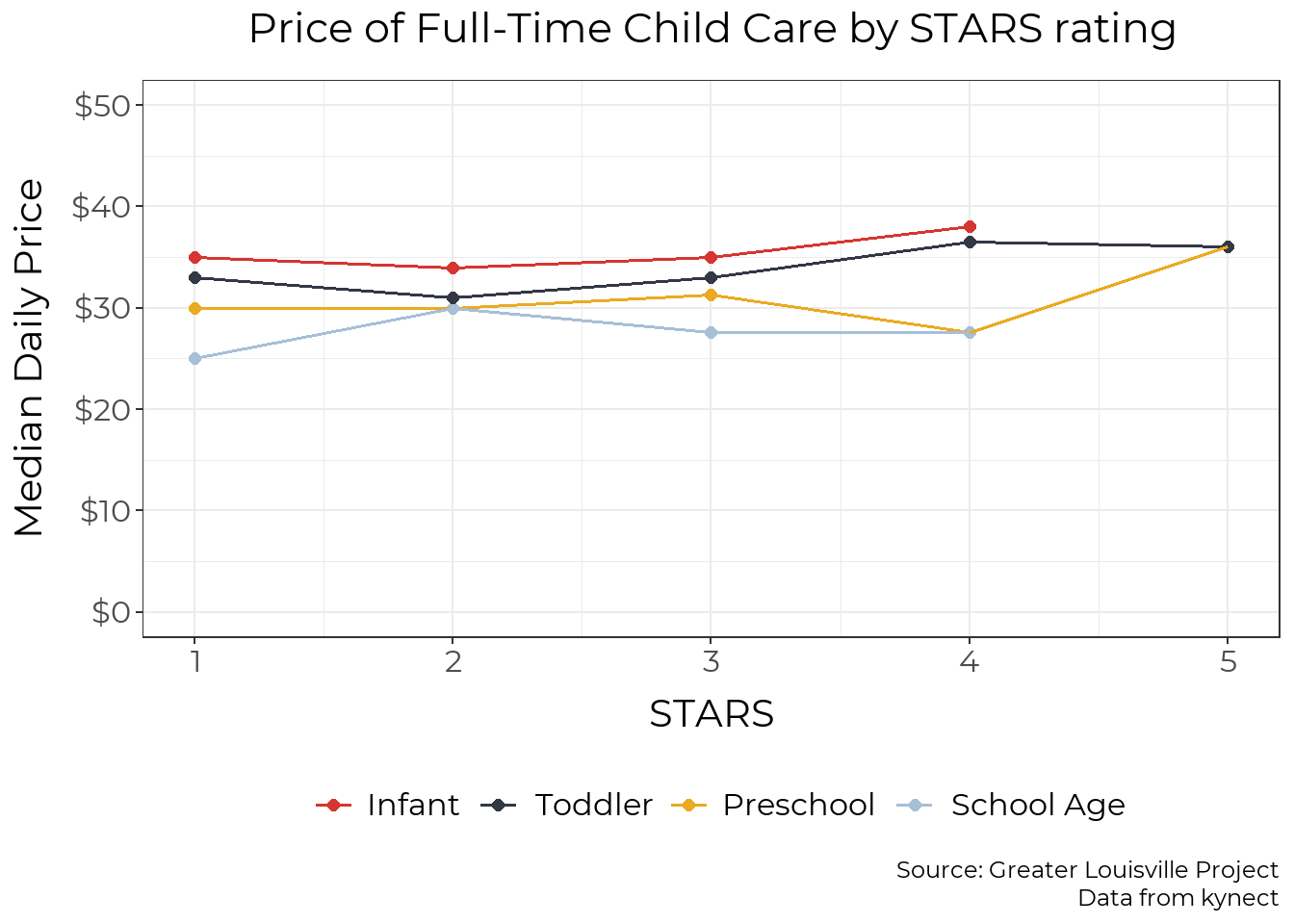
Location
Provider map
The map below shows the location of the 395 licensed child care providers throughout the city. Hover over the map to see provider information.
The size of the circle indicates the number of licensed slots, and the color of the circle indicates the provider’s Kentucky All STARS quality rating, a measure of quality based on family engagement, classroom quality, and staff qualifications. STARS level one is the default level indicating the provider is in good standing, and providers can choose to be evaluated to potentially earn a higher rating. The data does not distinguish between providers who have gone unrated and providers who earned a level one rating. Providers might not feel the need to confirm their quality with a state evaluation—for example, a school-based child care provider might have a good reputation among parents and not consider a STARS rating to be worthwhile. So, while providers at STARS level one can have varying levels of quality, providers at levels two and above have been evaluated and certified to meet certain standards.
Providers of all ratings can be found throughout the city. Looking at the distribution of quality ratings by neighborhood, there are no discernible trends. A larger issue is the general access to quality care: there are only three 5-STAR providers in Louisville, and only 107 out of 395 providers have more than one star.
# Geocode providers

# Break information into individual pieces for best results
provider_information_addressed <- provider_information %>%
  mutate(
    street = str_extract(Location, ".*?(?=,)"),
    city = str_extract(Location, "(?<=, )\\w*(?=, KY)"),
    county = "Jefferson",
    state = "KY",
    postalcode = str_sub(Location, -5))

# Use free default providers first (Census and OSM)
pi_cascade <- provider_information_addressed %>%
  geocode(
    street = street,
    city = city,
    state = state,
    postalcode = postalcode,
    method = "cascade")

# Fill in missings with Geocodio (free up to 2,500 per day)

Sys.setenv(GEOCODIO_API_KEY = "########")
#pw: "###########"

pi_fails <- pi_cascade %>%
  filter(is.na(lat)) %>%
  select(-lat, -long, -geo_method)

pi_fails %<>%
  geocode(
    street = street,
    city = city,
    state = state,
    postalcode = postalcode,
    method = "geocodio") %>%
  mutate(geo_method = "geocodio")

pi_fails %<>%
  mutate(geo_method = "geocodio")

pi_cascade %<>%
  filter(!is.na(lat)) %>%
  bind_rows(pi_fails)

pi_cascade %<>% filter(CLR != "L355501")

save(pi_cascade, file = "raw_data/provider_locations.RData")
load("raw_data/provider_locations.RData")
provider_map <- st_as_sf(pi_cascade,
coords = c("long", "lat"),
crs = 4326)
pi_cascade %<>%
mutate(
offerings = paste0(
if_else(Infant, "Infant, ", ""),
if_else(Toddler, "Toddler, ", ""),
if_else(Preschool, "Preschool, ", ""),
if_else(School, "School-age", "")),
offerings = str_remove(offerings, ", $"),
line1 = Name,
line2 = paste0("STARS level: ", if_else(is.na(STARS), "unknown",
as.character(STARS))),
line3 = paste0("Capacity: ", Capacity),
line4 = paste0("Age range: ", offerings),
)
provider_labels <-
sprintf("%s<br/>%s<br/>%s<br/>%s",
pi_cascade$line1,
pi_cascade$line2,
pi_cascade$line3,
pi_cascade$line4) %>%
lapply(htmltools::HTML)
pi_cascade %<>%
mutate(
stars_color = viridis(5)[STARS],
STARS = replace_na(STARS, "unknown"),
stars_color = replace_na(stars_color, "#505050"))
m <- leaflet(pi_cascade) %>%
addTiles() %>%
addCircleMarkers(lng = ~long, lat = ~lat,
radius = ~sqrt(Capacity),
color = ~stars_color,
label = provider_labels,
opacity = 0.8,
weight = 2,
labelOptions = labelOptions(style =
list("font-weight" = "normal",
"font-family" = "Montserrat",
padding = "3px 8px"),
textsize = "15px",
direction = "auto")) %>%
addPolygons(data = st_transform(filter(map_county, FIPS == "21111"), 4326),
fill = F, weight = 2, color = "black") %>%
addLegend(title = "STARS rating", labels = c(1:5, "unknown"), colors = c(viridis(5), "#505050"))
m %<>% htmlwidgets::prependContent(html_fix)
htmlwidgets::saveWidget(m, file = "index_maps/locations.html")
knitr::include_url("index_maps/locations.html")Providers by Neighborhood
Unlike STAR ratings, there are patterns in terms of the distribution of child care slots throughout Louisville. The map below shows the number of child care slots available to children ages 0 to 4 by neighborhood. The highest availability is located around Butchertown, Clifton, Crescent Hill, and Downtown. This likely reflects the large number of people who commute to work in this area and use nearby child care. These neighborhoods are the only ones where there are more slots available than children who live there.
The lowest availability of child care is in neighborhoods at the very Southwest and West of the city: Fairdale and Valley Station in South Louisville, and Chickasaw, Shawnee, and Portland in West Louisville.
map_nh <- st_transform(map_nh, 4326)

provider_nh <- st_join(provider_map, map_nh, join = st_within)

provider_nh %<>%
  group_by(neighborhood) %>%
  summarise(seats = sum(infant_est + toddler_est + preschool_est))

child_pop <- poverty_nh %>%
  filter(year == max(year),
         sex == "total",
         race %in% c("total", "white"),
         var_type == "population") %>%
  select(neighborhood, race, poverty_under_5) %>%
  pivot_wider(names_from = "race", values_from = "poverty_under_5") %>%
  mutate(
    percent_nonwhite = (total - white) / total * 100)

provider_nh_summary <- provider_nh %>%
  st_drop_geometry() %>%
  left_join(child_pop, by = "neighborhood") %>%
  mutate(seats_per = seats / total) %>%
  transmute(
    Neighborhood = neighborhood,
    `Estimated Seats` = seats,
    `Seats per child` = seats_per,
    `Percent Nonwhite` = percent_nonwhite)

provider_nh_map <- map_nh %>%
  left_join(provider_nh_summary, by = c("neighborhood" = "Neighborhood"))

ggplot(provider_nh_map) +
  geom_sf(aes(fill=`Seats per child`), color = "white") +
  scale_fill_viridis(na.value = "grey", name = "Slots per child") +
  theme_bw(base_size = 22) +
  theme(plot.caption = element_text(lineheight = .5)) +
  theme(text = element_text(family = "Montserrat"),
        panel.grid = element_blank(),
        axis.text = element_blank(),
        axis.ticks = element_blank(),
        axis.title = element_blank(),
        panel.border = element_blank()) +
  labs(title = "Child Care Slots per Child Ages 0 - 4",
       subtitle = "Includes Infants, Toddlers, and Preschool Slots",
       caption_text = "Source: Greater Louisville Project
                       Data from kynect and ACS Table B17001") +
  theme(plot.caption = element_text(lineheight = .5)) +
  theme(
    panel.background = element_rect(fill = "transparent", color = NA), # bg of the panel
    plot.background = element_rect(fill = "transparent", color = NA), # bg of the plot
    legend.background = element_rect(fill = "transparent", color = "transparent"), # get rid of legend bg
    legend.box.background = element_rect(fill = "transparent", color = "transparent"), # get rid of legend panel bg
    legend.key = element_rect(fill = "transparent",colour = NA))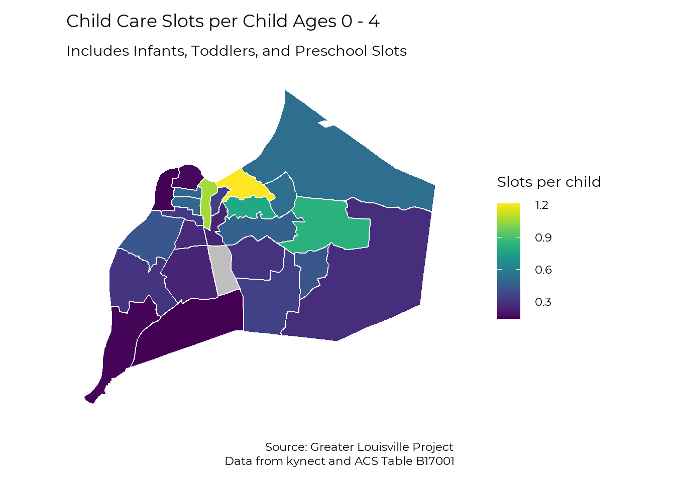
Neighborhoods by Race and Licensed Slots
The neighborhoods with the highest availability of child care tend to be neighborhoods with a predominantly white population. As a result, parents of children who are Black, Hispanic, Indigenous, Asian, and other races are more likely to have difficulty accessing child care due to where they live.
On the graph below, neighborhoods with a higher percentage of children who are white are to the left, and neighborhoods with more children who are Black, Hispanic, Indigenous, Asian, and other races are to the right.
avg_annotation1 <- list(
  x = 90,
  y = mean(provider_nh_summary$`Estimated Seats`) + 150,
  xref = 'x', yref = 'y',
  text = "City Average",
  showarrow = FALSE)

avg_annotation2 <- list(
  x = 90,
  y = sum(provider_nh_summary$`Estimated Seats`) / sum(child_pop$total) + 0.045,
  xref = 'x', yref = 'y',
  text = "City Average",
  showarrow = FALSE)

plot_ly(provider_nh_summary) %>%
  add_markers(x = ~`Percent Nonwhite`, y = ~`Estimated Seats`,
              text = provider_nh_summary$Neighborhood,
              marker = list(color = '#d63631', size = 10),
              hoverinfo = 'text',
              visible = TRUE) %>%
  add_segments(x = 0, xend = 100,
               y = mean(provider_nh_summary$`Estimated Seats`),
               yend = mean(provider_nh_summary$`Estimated Seats`),
               line = list(color = '#323844', width = 1, dash = 'dash'),
               visible = TRUE) %>%
  add_markers(x = ~`Percent Nonwhite`, y = ~`Seats per child`,
              text = provider_nh_summary$Neighborhood,
              marker = list(color = '#d63631', size = 10),
              hoverinfo = 'text',
              visible = FALSE) %>%
  add_segments(x = 0, xend = 100,
               y = sum(provider_nh_summary$`Estimated Seats`) / sum(child_pop$total),
               yend = sum(provider_nh_summary$`Estimated Seats`) / sum(child_pop$total),
               line = list(color = '#323844', width = 1, dash = 'dash'),
               visible = FALSE) %>%
  layout(
    font = list(family = "Montserrat"),

    title = "Estimated Child Care Provider Slots by Race",

    xaxis = list(title = "Percent of Children Age 0-4 Who Are BIPOC"),
    yaxis = list(title = "Total Estimated Slots", rangemode = "tozero"),
    showlegend = FALSE,
    updatemenus = list(
      list(
        active = 0,
        x = 0.95,
        y = 0.85,
        buttons = list(
          list(label = "Total Estimated Slots",
               method = "update",
               args = list(list(visible = list(TRUE, TRUE, FALSE, FALSE)),
                           list(yaxis = list(title = "Total Estimated Slots",
                                             rangemode = "tozero"),
                                annotations = list(avg_annotation1, c())))),
          list(label = "Estimated Slots per child",
               method = "update",
               args = list(list(visible = list(FALSE, FALSE, TRUE, TRUE)),
                           list(yaxis = list(title = "Estimated Slots per Child",
                                             rangemode = "tozero"),
                                annotations = list(c(), avg_annotation2))))))))
Hours
Another barrier to child care access is the hours during which providers are open. The vast majority of child care providers are open between 6am and 6pm Monday through Friday, so the availability of child care is limited outside of traditional first shift hours. Black and Brown workers are more likely to work irregular hours, weekends, and second or third shift when childcare is less available.
hours_info <- provider_hours %>%
  left_join(provider_information) %>%
  select(CLR, Capacity, Day, open_time, close_time)

all_day_seats <- hours_info %>%
  filter(abs(open_time - close_time) <= 1)

hours_info %<>%
  anti_join(all_day_seats, by = c("CLR", "Day"))

all_day_seats %<>%
  group_by(Day) %>%
  summarise(seats = sum(Capacity))

for(day in c("Monday", "Tuesday", "Wednesday", "Thursday", "Friday", "Saturday", "Sunday")) {
  for(time in seq(0, 24, by = 0.25)) {

    capacity <- hours_info %>%
      filter(
        Day %in% day, # Filter to day

        # Time is greater than opening time OR
        #   if close time is post midnight (less than opening time), less than close time
        time >= open_time | (close_time < open_time & time <= close_time),

        # Time is greater than opening time OR
        #   close time is post midnight
        time <= close_time | close_time < open_time) %>%
      summarise(seats = sum(Capacity)) %>%
      pull(seats)

    temp = c("Day" = day, "Time" = time, "Seats" = capacity)

    seat_summary <- assign_row_join(seat_summary, temp)

  }
}

seat_summary %<>%
  mutate(
    Time = as.numeric(Time),
    Seats = as.numeric(Seats)) %>%
  left_join(all_day_seats, by = "Day") %>%
  mutate(Seats = Seats + seats) %>%
  select(-seats) %>%
  mutate(day_category =
           case_when(Day %in% c("Monday", "Tuesday", "Wednesday", "Thursday", "Friday") ~ "Monday - Friday",
                     Day == "Saturday" ~ "Saturday",
                     Day == "Sunday" ~ "Sunday")) %>%
  group_by(Time, day_category) %>%
  summarise(Seats = round(mean(Seats), 0), .groups = "drop") %>%
  filter(Time != 24) %>%
  mutate(
    hour = trunc(Time),
    minute = str_pad((Time - hour) * 60, 2, "left", "0"),
    suffix = if_else(hour %in% 12:23, "PM", "AM"),
    hour = case_when(hour %in% c(0, 12, 24) ~ 12,
                     hour %in% 1:11 ~ hour,
                     hour %in% 13:23 ~ hour - 12),
    time = paste0(hour, ":", minute, " ", suffix),
    time_label = factor(Time, levels = Time, labels = time, ordered = TRUE))

seat_summary %<>%
  select(
    `Day of the Week` = day_category,
    time_label,
    Seats) %>%
  pivot_wider(names_from = `Day of the Week`, values_from = Seats)

plot_ly(seat_summary,
        hoverinfo = 'text') %>%
  add_trace(x = ~time_label, y = ~`Monday - Friday`,
            name = "Monday - Friday", type = "scatter", mode = "lines",
            line = list(color = '#d63631', width = 4),
            hoverinfo = 'text',
            text = paste0(seat_summary$time_label,
                          "<br>Slots available: ",
                          scales::comma(seat_summary$`Monday - Friday`, accuracy = 1),
                          "<br>Percent available: ",
                          scales::percent(seat_summary$`Monday - Friday` / 31597,
                                          accuracy = 0.1))) %>%
  add_trace(x = ~time_label, y = ~Saturday, name = "Saturday", type = "scatter", mode = "lines",
            line = list(color = '#323844', width = 4),
            hoverinfo = 'text',
            text = paste0(seat_summary$time_label,
                          "<br>Slots available: ",
                          scales::comma(seat_summary$Saturday, accuracy = 1),
                          "<br>Percent available: ",
                          scales::percent(seat_summary$Saturday / 31597,
                                          accuracy = 0.1))) %>%
  add_trace(x = ~time_label, y = ~Sunday, name = "Sunday", type = "scatter", mode = "lines",
            line = list(color = '#eaab21', width = 4),
            hoverinfo = 'text',
            text = paste0(seat_summary$time_label,
                          "<br>Slots available: ",
                          scales::comma(seat_summary$Sunday, accuracy = 1),
                          "<br>Percent available: ",
                          scales::percent(seat_summary$Sunday / 31597,
                                          accuracy = 0.1))) %>%
  layout(
    font = list(family = "Montserrat"),
    title = "Licensed Child Care Provider Slots by Day and Time",
    xaxis = list(title = "Time of Day",
                 nticks = 12,
                 tickangle = 90),
    yaxis = list(title = "Slots available"),
    legend = list(x = 0.8, y = 1))
Compensation of Child Care Workers
Ranking
A major factor restricting the expansion of child care, especially high-quality care, is relatively low wages in the child care field. In 2019, the median hourly wages for Louisville child care workers was $9.78.
read_and_prep <- function(file_path) {
  df <- readxl::read_excel(file_path) %>%
    janitor::clean_names() %>%
  mutate(MSA = as.numeric(area),
         h_median = as.numeric(h_median)) %>%
  filter(MSA %in% c(24340, 41180, 36420, 46140, 24860, 28940, 13820, 31140, 26900,
                        28140, 36540, 24660, 16740, 18140, 17140, 34980, 32820) &
           occ_title %in% c("Childcare Workers", "Child care workers")) %>%
  select(MSA, tot_emp, h_mean, a_mean, h_median, a_median) %>%
  mutate(city = case_when(
    MSA == 24340 ~ "Grand Rapids",
    MSA == 41180 ~ "St. Louis",
    MSA == 36420 ~ "Oklahoma City",
    MSA == 46140 ~ "Tulsa",
    MSA == 24860 ~ "Greenville",
    MSA == 28940 ~ "Knoxville",
    MSA == 13820 ~ "Birmingham",
    MSA == 31140 ~ "Louisville",
    MSA == 26900 ~ "Indianapolis",
    MSA == 28140 ~ "Kansas City",
    MSA == 36540 ~ "Omaha",
    MSA == 24660 ~ "Greensboro",
    MSA == 16740 ~ "Charlotte",
    MSA == 18140 ~ "Columbus",
    MSA == 17140 ~ "Cincinnati",
    MSA == 34980 ~ "Nashville",
    MSA == 32820 ~ "Memphis",
    TRUE ~ NA_character_
  ))

return(df)

}

df19 <- read_and_prep("bls_data/MSA_M2019_dl.xlsx") %>%
  mutate(year = 2019)

ranking(df19,
        "h_median",
        text_size = 2,
        plot_title = "Median Wages for Child Care Workers, 2019",
        year = 2019,
        caption_text = "Source: Greater Louisville Project
                        Data from the Bureau of Labor Statistics",
        y_title = "Hourly Wage",
        FIPS_df = FIPS_df)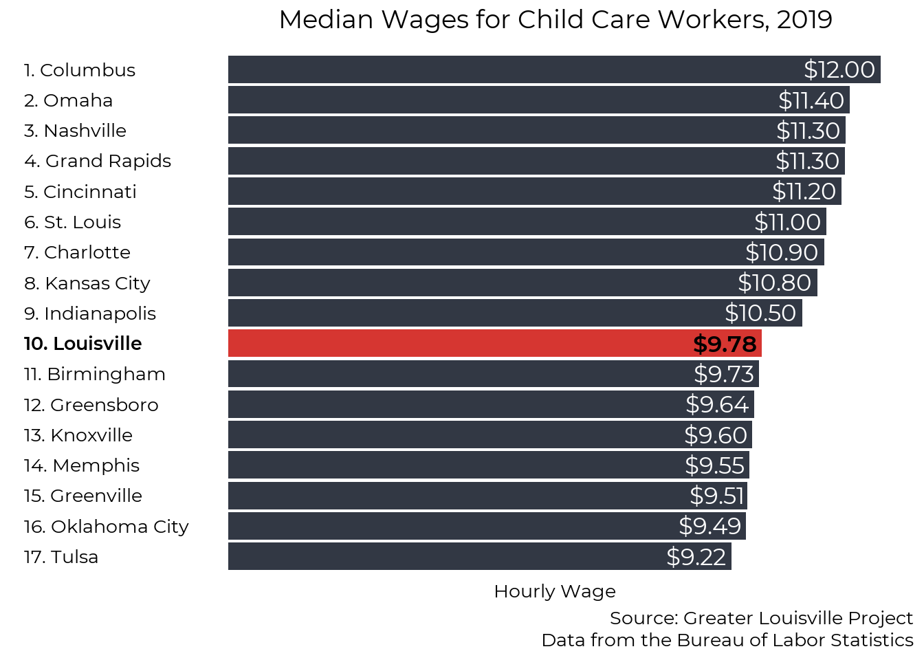
Trend
The relatively low pay rate is around the 25th percentile of Louisville’s peer cities. After adjusting for inflation, median wages for child care workers have fallen since 2010.
df18 <- read_and_prep("bls_data/MSA_M2018_dl.xlsx") %>%
  mutate(year = 2018)

df17 <- read_and_prep("bls_data/MSA_M2017_dl.xlsx") %>%
  mutate(year = 2017)

df16 <- read_and_prep("bls_data/MSA_M2016_dl.xlsx") %>%
  mutate(year = 2016)

df15 <- read_and_prep("bls_data/MSA_M2015_dl.xlsx") %>%
  mutate(year = 2015)

df14 <- read_and_prep("bls_data/MSA_M2014_dl.xlsx") %>%
  mutate(year = 2014)

df13 <- read_and_prep("bls_data/MSA_M2013_dl_1_AK_IN.xls") %>%
  bind_rows(read_and_prep("bls_data/MSA_M2013_dl_2_KS_NY.xls")) %>%
  bind_rows(read_and_prep("bls_data/MSA_M2013_dl_3_OH_WY.xls")) %>%
  mutate(year = 2013)

df12 <- read_and_prep("bls_data/MSA_M2012_dl_1_AK_IN.xls") %>%
  bind_rows(read_and_prep("bls_data/MSA_M2012_dl_2_KS_NY.xls")) %>%
  bind_rows(read_and_prep("bls_data/MSA_M2012_dl_3_OH_WY.xls")) %>%
  mutate(year = 2012)

df11 <- read_and_prep("bls_data/MSA_M2011_dl_1_AK_IN.xls") %>%
  bind_rows(read_and_prep("bls_data/MSA_M2011_dl_2_KS_NY.xls")) %>%
  bind_rows(read_and_prep("bls_data/MSA_M2011_dl_3_OH_WY.xls")) %>%
  mutate(year = 2011)

df10 <- read_and_prep("bls_data/MSA_M2010_dl_1.xls") %>%
  bind_rows(read_and_prep("bls_data/MSA_M2010_dl_2.xls")) %>%
  bind_rows(read_and_prep("bls_data/MSA_M2010_dl_3.xls")) %>%
  mutate(year = 2010)

df09 <- read_and_prep("bls_data/MSA_M2009_dl_1.xls") %>%
  bind_rows(read_and_prep("bls_data/MSA_M2009_dl_2.xls")) %>%
  bind_rows(read_and_prep("bls_data/MSA_M2009_dl_3.xls")) %>%
  mutate(year = 2009)

df08 <- read_and_prep("bls_data/MSA_M2008_dl_1.xls") %>%
  bind_rows(read_and_prep("bls_data/MSA_M2008_dl_2.xls")) %>%
  bind_rows(read_and_prep("bls_data/MSA_M2008_dl_3.xls")) %>%
  mutate(year = 2008)

df07 <- read_and_prep("bls_data/MSA_May2007_dl_1.xls") %>%
  bind_rows(read_and_prep("bls_data/MSA_May2007_dl_2.xls")) %>%
  bind_rows(read_and_prep("bls_data/MSA_May2007_dl_3.xls")) %>%
  mutate(year = 2007)

df06 <- read_and_prep("bls_data/MSA_may2006_dl_1.xls") %>%
  bind_rows(read_and_prep("bls_data/MSA_may2006_dl_2.xls")) %>%
  bind_rows(read_and_prep("bls_data/MSA_may2006_dl_3.xls")) %>%
  mutate(year = 2006)

df05 <- read_and_prep("bls_data/MSA_may2005_dl_1.xls") %>%
  bind_rows(read_and_prep("bls_data/MSA_may2005_dl_2.xls")) %>%
  bind_rows(read_and_prep("bls_data/MSA_may2005_dl_3.xls")) %>%
  mutate(year = 2005)

#MSA codes all change in 2004

df_t <- bind_rows(df19, df18, df17, df16, df15, df14, df13, df12, df11, df10, df09, df08, df07, df06, df05)

#inflate to 2019 dollars based on CPI
df_cpi <- tibble(
  year = 2005:2019,
  cpi_value = c(195.292, 201.592, 207.342, 215.303, 214.537, 218.056, 224.939, 229.594, 232.957,
                236.736, 237.017, 240.007, 245.120,
                251.107, 255.657)
) %>%
  mutate(multiplier = max(cpi_value)/ cpi_value) #scale to 2019 dollars

df_t <- left_join(df_t, df_cpi, by = "year")

df_t <- df_t %>%
  mutate(h_median = h_median * multiplier)

trend_cc(df_t,
         "h_median",
         plot_title = "Median Hourly Wages for Child Care Workers",
         y_title = "Hourly Wage",
         caption_text = "Source: Greater Louisville Project
                         Data from the Bureau of Labor Statistics")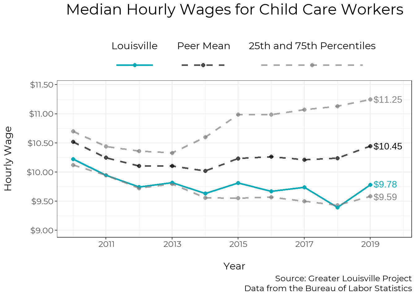
Child Health
Child health is important for healthy child development and future success. Physical and mental health are incredibly important in their own right, and they also enable children to enter school ready to learn. This section discusses adverse childhood experiences and food insecurity, two factors that can have detrimental impacts on child well-being.
Adverse Childhood Experiences
Adverse childhood experiences are traumatic events that occur in childhood. If you would prefer to skip past this section, click “Child Food Security” in the sidebar.
Adverse Childhood Experiences (ACEs) include forms of abuse, neglect, and household dysfunction. According to the CDC, “ACEs can have lasting, negative effects on health, well-being, and opportunity.” In 2018, 71% of Louisville adults reported experiencing one or more ACEs during their childhood.
ACEs data was collected by the Kentucky Behavioral Risk Factor Survey using phone interviews throughout 2018. The total number of ACEs a person has experienced is considered their ACE score—to understand the questionnaire and find your ACE score, you can click here.
Kentucky Department for Public Health (KDPH) and the Centers for Disease Control and Prevention (CDC). Kentucky Behavioral Risk Factor Survey Data – Adverse Childhood Experiences 2015&2018. Frankfort, Kentucky: Cabinet for Health and Family Services, Kentucky Department for Public Health, [2018].
Impact of ACEs
Louisville adults who have experienced a high number of ACEs report much higher numbers of chronic disease than those who experienced no ACEs. The chart below compares the prevalence of several health conditions among the two groups. The data is based on the health status of current adults based on the number of ACEs they report having experienced as a child.
Compared to adults who experienced no ACEs, adults who experienced a high number of ACEs are 6.5 times as likely to be a current smoker, 2.2 times as likely to report poor health status, 6.3 times as likely to have had a heart attack, and 3.9 times as likely to experience depression.
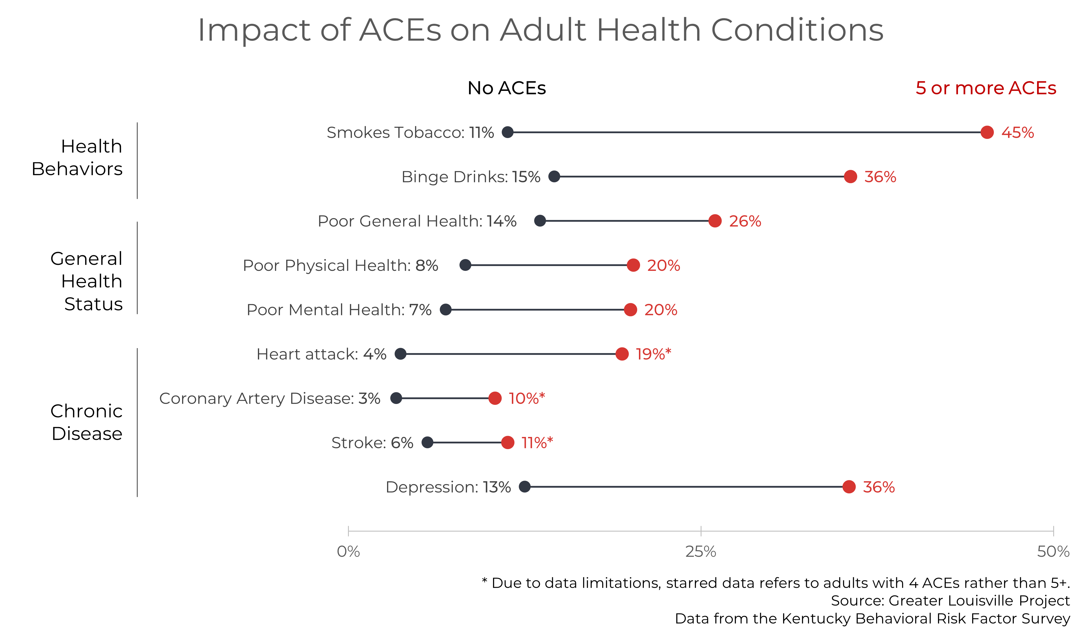
Prevalance of ACEs
ACE Scores
The number of ACEs a person has experienced is considered their ACE score. The 2018 KyBRFS survey asked about nine different kinds of ACEs. In 2018, 71% of adults in Louisville reported experiencing at least one ACE when they were a child. Higher numbers of ACEs are associated with greater prevalence of risk factors and chronic disease.
ace_prevalance <- tibble(
  number = c(0:4, "5+"),
  percent = c(29, 20.8, 17.8, 10, 10, 12.4)) %>%
  mutate(
    number = factor(number, levels = rev(c(0:4, "5+")), ordered = T),
    label_text = scales::percent(percent, scale = 1),
    ypos = cumsum(percent) - 0.5 * percent)

text_size = 2

p <- ggplot(ace_prevalance, aes(x=factor(1), y=percent))

p = p + guides(fill = FALSE, color = FALSE, alpha = FALSE)

p <- p +
  geom_bar(aes(alpha = number),
           stat = "identity",
           width = 1,
           size = text_size,
           fill = "#d63631") +
  scale_alpha_manual(
    name = "Number of ACEs",
    breaks = c(0:4, "5+"), values = seq(0.2, 1, length.out = 6)) +
  coord_polar("y") +
  theme_void() +
  geom_text(aes(label = label_text, family = "Montserrat", x = 1.2),
            color = "black", size = 12, position = position_stack(vjust = 0.5))

p <- p + theme(text = element_text(family = "Montserrat"),
               plot.title = element_text(size = 14 * text_size, hjust = 0.5, margin = margin(b = 10, unit = "pt")),
               legend.text = element_blank(),
               legend.title = element_blank(),
               plot.caption = element_text(size = 10 * text_size, lineheight = 0.5))
               # legend.text = element_text(size = 12 * text_size, lineheight = 0.5),
               # legend.title = element_text(size = 12 * text_size))

p <- p + labs(title = " ACE scores for Louisville Adults, 2018",
              caption = "Source: Greater Louisville Project
                         Data from the Kentucky Behavioral Risk Factor Survey")

p <- p +
  theme(
    panel.background = element_rect(fill = "transparent", color = NA), # bg of the panel
    plot.background = element_rect(fill = "transparent", color = NA), # bg of the plot
    legend.background = element_rect(fill = "transparent", color = "transparent"), # get rid of legend bg
    legend.box.background = element_rect(fill = "transparent", color = "transparent"), # get rid of legend panel bg
    legend.key = element_rect(fill = "transparent",colour = NA))

p <- p + geom_text(aes(label = number,
                       family = "Montserrat",
                       x = 1.6),
            color = "black", size = 12,
            position = position_stack(vjust = 0.5))

p
Type of ACEs
The most common ACE Louisville adults report experiencing as a child is divorce among their parents, followed by a drinking problem in the household. Over one quarter of adults reported experiencing verbal abuse as a child.
ace_types <- tibble(
  category = c(rep("abuse", 3), rep("dysfunction", 6)),
  type = c("physical_abuse", "sexual_abuse", "verbal_abuse",
           "incarcerated_hh_member", "drug_problem", "drinking_problem",
           "witness_domestic_violence", "mentally_ill_hh_member", "divorced_parents"),
  percent = c(12.5, 15.4, 28.2, 9.7, 16.9, 31.6, 20.5, 26.1, 41.8))

ace_types %<>%
  mutate(type = factor(type,
                       levels = c("verbal_abuse",
                                  "sexual_abuse",
                                  "physical_abuse",
                                  "divorced_parents",
                                  "drinking_problem",
                                  "mentally_ill_hh_member",
                                  "witness_domestic_violence",
                                  "drug_problem",
                                  "incarcerated_hh_member"),
                       labels = c("Verbal abuse",
                                  "Sexual abuse",
                                  "Physical abuse",
                                  "Divorced Parents",
                                  "Drinking problem in household",
                                  "Mentally ill household member",
                                  "Witnessed domestic violence",
                                  "Drug problem in household",
                                  "Incarcerated household member"),
                       ordered = TRUE))

ace_types %<>%
  mutate(label_text = scales::percent(percent, scale=1, accuracy = 1))

text_size = 2

p <- ggplot(ace_types, aes(type, percent))

p = p + guides(fill = FALSE, color = FALSE)

p <- p +
  geom_bar(stat = "identity",
           size = text_size,
           fill = "#d63631") +
  coord_flip(clip="off") +
  ggthemes::theme_tufte()

p <- p + theme(text = element_text(family = "Montserrat"),
               plot.title = element_text(size = 12.5 * text_size, hjust = 0.5, margin = margin(b = 10, unit = "pt")),
               axis.text.y = element_text(hjust = 0,
                                          size = 10 * text_size),
               axis.title.x = element_text(size = 10 * text_size),
               axis.title.y = element_text(size = 10 * text_size),
               axis.ticks = element_blank(),
               axis.text.x = element_blank(),
               plot.caption = element_text(size = 10 * text_size, lineheight = 0.5))

# p <- p +
#   labs(subtitle = subtitle_text) +
#   theme(plot.subtitle = element_text(hjust = 0.5, size = 10 * text_size))

# Add remaining text
p <- p + labs(title = "Prevalance of ACEs among Louisville adults, 2018",
              x = "",
              caption = "Souce: Greater Louisville Project
                         Data from the Kentucky Behavioral Risk Factor Survey")

p <- p +
  theme(
    panel.background = element_rect(fill = "transparent", color = NA), # bg of the panel
    plot.background = element_rect(fill = "transparent", color = NA), # bg of the plot
    legend.background = element_rect(fill = "transparent", color = "transparent"), # get rid of legend bg
    legend.box.background = element_rect(fill = "transparent", color = "transparent"), # get rid of legend panel bg
    legend.key = element_rect(fill = "transparent",colour = NA))

p <- p + geom_text(aes(label = label_text,
                       family = "Montserrat Bold"),
                   size = 4.5 * text_size,
                   color = "black",
                   hjust = 1.1)

p
ACEs by Race
The most recent national data from the National Survey of Children’s Health shows that children who are Hispanic or Black are more likely to have experienced one or more ACEs than other children. While we have some local data for children of different races, it is limited and highly variable from year to year. The original ACEs questionnaire mostly measures trauma that occurs in the home, and it excludes many kinds of trauma that are most likely to affect Black and Brown children, such as racial discrimination from peers, experiences with community violence, and family separation.
There are various proposals to create a more comprehensive “expanded” or “culturally-informed” ACEs measure. Some suggestions include adding questions about community experiences, such as witnessing violence or living in unsafe neighborhoods. Proposals also include collecting more data on experiences with racism, including discrimination, stigma, and historical trauma. Racism can not only be a form of trauma; it can amplify other kinds of trauma as well.
Child Food Security
According to Feeding America, “research shows an association between food insecurity and delayed development in young children; risk of chronic illnesses like asthma and anemia; and behavioral problems like hyperactivity, anxiety and aggression in school-age children.” Child food security data comes from Feeding America’s Mind the Meal Gap program.
Trend
From 2014 to 2018, Louisville saw a slight decline in child food insecurity. However, child food insecurity increased by 40% in Louisville from 2018 to October of 2020.
# Read in food insecurity data from Mind the Meal Gap
dinner_time <- function(folder, starting_year){

  wd <- getwd()
  directory <- paste0(wd, "/", folder)
  file_names <- list.files(directory)

  # Read file for each year
  for (y in starting_year:2018){

    # Create parameters to read in sheet based on the year
    file_path <- paste0(wd, "/", folder, "/", file_names[y-2008])

    sheet_name <- case_when(
      y %in% 2009:2010 ~ "County",
      y %in% 2011:2018 ~ paste0(y, " County"))

    skip_num <- case_when(
      y %in% 2009:2017 ~ 0,
      y %in% 2018 ~ 1)

    df <- readxl::read_xlsx(file_path, sheet = sheet_name, skip = skip_num)

    # Create variables names based on the year
    food_insecure_var <- paste0(y, " Food Insecurity Rate")
    food_insecure_num_var <- paste0("# of Food Insecure Persons in ", y)
    child_food_insecure_var <- paste0(y, " Child food insecurity rate")
    child_food_insecure_num_var <- paste0("# of Food Insecure Children in ", y)
    insecure_FRL <- paste0("% food insecure children in HH w/ HH incomes below 185 FPL in ", y)
    insecure_non_FRL <- paste0("% food insecure children in HH w/ HH incomes above 185 FPL in ", y)

    # Tidy data frame
    df %<>%
      transmute(
        FIPS = str_pad(FIPS, 5, "left", "0"),
        year = y,
        food_insecurity = .data[[food_insecure_var]],
        food_insecurity_num = .data[[food_insecure_num_var]],
        child_food_insecurity = .data[[child_food_insecure_var]],
        child_food_insecurity_num = .data[[child_food_insecure_num_var]],

        low_threshold = `Low Threshold in state`,
        low_threshold_type = `Low Threshold Type`,
        high_threshold = `High Threshold in state`,
        high_threshold_type = `High Threshold Type`,
        under_low = `% FI ≤ Low Threshold`,
        between = `% FI Btwn Thresholds`,
        above = `% FI > High Threshold`,
        child_below_FRL = .data[[insecure_FRL]],
        child_above_FRL = .data[[insecure_non_FRL]])

    output <- assign_row_join(output, df)
  }
  output
}

feeding_america <- dinner_time("raw_data/Map the Meal Gap data", starting_year = 2012)
feeding_america_covid <- readxl::read_xlsx("raw_data/Projections data (revised Oct. 2020)/The Impact of Coronavirus on Food Insecurity Update 10.2020.xlsx", sheet = "County")

feeding_america_covid %<>%
  transmute(
    FIPS = str_pad(FIPS, 5, "left", "0"),
    year = 2020,
    food_insecurity = `[Revised Projections – Oct 2020] \r\n2020 Food Insecurity  %`,
    food_insecurity_num = `[Revised Projections – Oct 2020] \r\n2020 Food Insecurity #`,
    child_food_insecurity = `[Revised Projections – Oct 2020] \r\n2020 Child Food Insecurity  %`,
    child_food_insecurity_num = `[Revised Projections – Oct 2020] \r\n2020 Child Food Insecurity #`)

feeding_america %<>%
  bind_rows(feeding_america_covid)

feeding_america %<>%
  pull_peers(FIPS_df = FIPS_df) %>%
  mutate(across(
    c(food_insecurity, child_food_insecurity, under_low, between, above, child_below_FRL, child_above_FRL),
    ~ . * 100))

feeding_america_1 <- feeding_america %>%
  stl_merge(food_insecurity_num, child_food_insecurity_num, method = "sum")

feeding_america_2 <- feeding_america %>%
  stl_merge(food_insecurity, under_low, between, above, method = "mean", weight_var = "food_insecurity_num")

feeding_america_3 <- feeding_america %>%
  stl_merge(child_food_insecurity, child_below_FRL, child_above_FRL, method = "mean", weight_var = "child_food_insecurity_num")

feeding_america_t = left_join(feeding_america_1, feeding_america_2) %>%
  left_join(feeding_america_3)

feeding_america_t %<>%
  mutate(pct_above_frl = child_above_FRL * child_food_insecurity / 100,
         pct_below_frl = (100 - child_above_FRL) * child_food_insecurity / 100)

trend_cc(feeding_america_t,
         "child_food_insecurity",
         plot_title = "Child Food Insecurity",
         caption_text = "Source: Greater Louisville Project
                         Data from Feeding America",
         y_title = "Percent",
         xmin = 2014, xmax = 2020)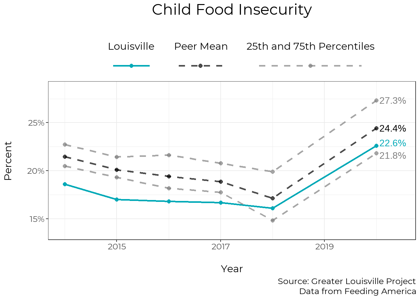
Ranking
While Louisville is toward the middle of its peer cities in child food Insecurity, more than 1 in 5 children are food insecure.
ranking(feeding_america_t,
        "child_food_insecurity",
        plot_title = "Child Food Insecurity, October 2020",
        caption_text = "Source: Greater Louisville Project
                        Data from Feeding America",
        year = 2020,
        order = "Ascending",
        text_size = 2,
        FIPS_df = FIPS_df)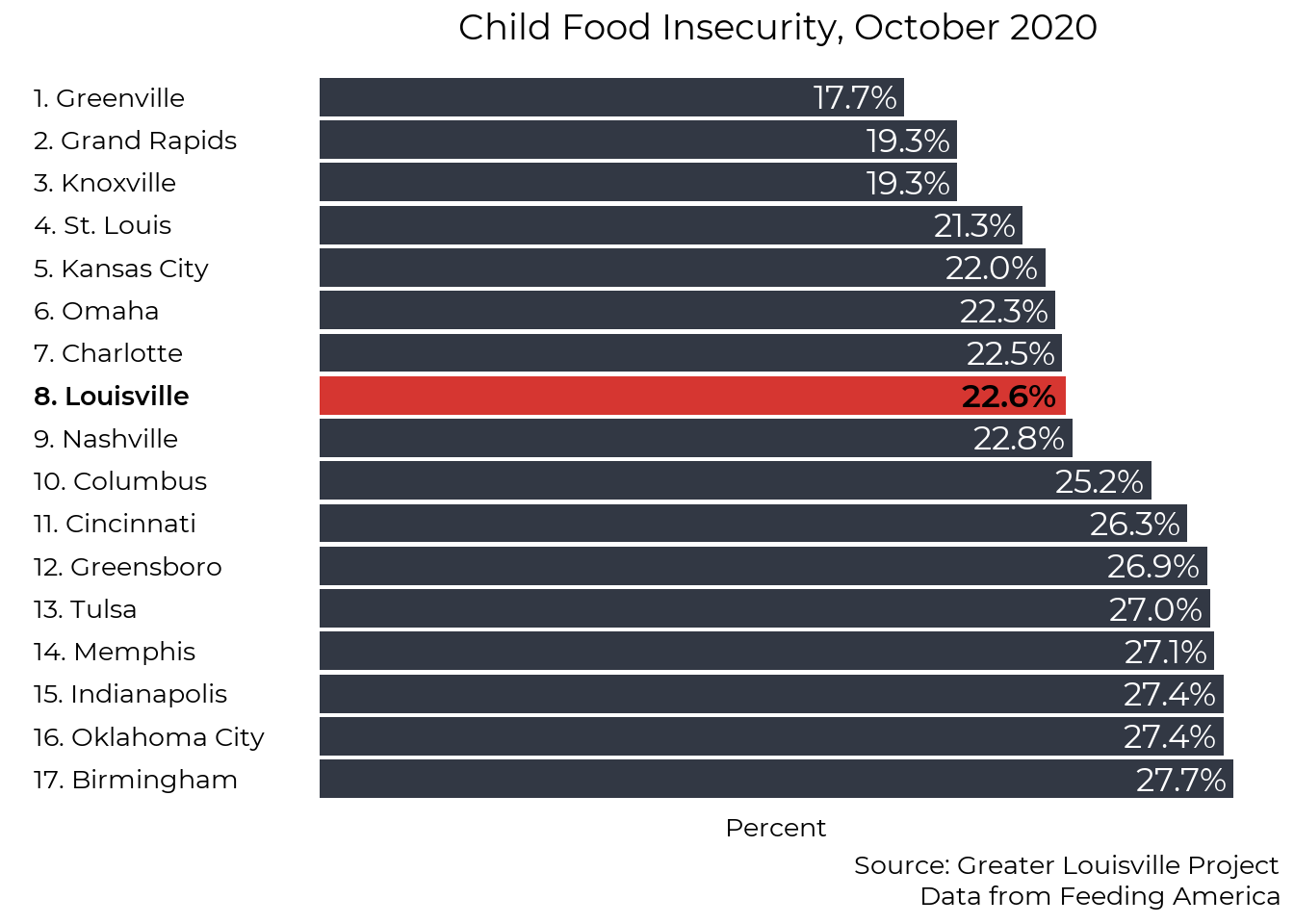
Breakdown by Program Eligibility
As of 2018, Feeding America estimated that most food-insecure children lived in families under 185% of the poverty line, meaning that they were generally eligible for programs like SNAP, WIC, and Free or Reduced School lunch.
Compared to cities with similar rates of overall child food insecurity, Louisville has a relatively low number of food insecure children who are eligible for food benefit programs and a relatively high number of food insecure children above this cutoff. This shows that food insecurity is prevalent in families with a wide range of incomes.
feeding_america_stack <- feeding_america_t %>%
  filter(year == 2018) %>%
  pull_peers(add_info = T, FIPS_df = FIPS_df) %>%
  filter(current == 1) %>%
  arrange(child_food_insecurity) %>%
  mutate(
    rank = row_number(),
    names = paste0(rank, ". ", city))

feeding_america_stack %<>%
  select(names, rank, city, pct_below_frl, pct_above_frl) %>%
  pivot_longer(pct_below_frl:pct_above_frl) %>%
  arrange(desc(name)) %>%
  group_by(city) %>%
  mutate(label_ypos = if_else(name == "pct_below_frl",
                              value[name == "pct_below_frl"],
                              sum(value)))

color_values <- c("#323844", "#d63631")
color_names <- c("Above 185% of poverty", "Below 185% of poverty")

feeding_america_stack$color <- "Below 185% of poverty"
feeding_america_stack$color[feeding_america_stack$name == "pct_above_frl"] <- "Above 185% of poverty"

feeding_america_stack$alpha = 0.9
feeding_america_stack$alpha[feeding_america_stack$city == "Louisville"] <- 1

# Create numeric labels
label_text <- feeding_america_stack$value %>%
  scales::percent(accuracy = 0.1, scale = 1, suffix = "%")


# Set text format, highlight and italicise Louisville text, highlight Louisville bar
feeding_america_stack$textcolor <- "#000000"
feeding_america_stack$textcolor[feeding_america_stack$name == "pct_above_frl"] <- "#000000"

feeding_america_stack$textfont <- "Montserrat"
feeding_america_stack$textfont[feeding_america_stack$city == "Louisville"] <- "Montserrat Bold"

label_color_names <- c("white", "black")
label_color_values <- c("#000000", "#ffffff")

feeding_america_stack$label_color <- "white"
feeding_america_stack$label_color[feeding_america_stack$name == "pct_above_frl"] <- "black"
#df$linecolor <- "#ffffff"
#df$linecolor[df$city == "Louisville"] <- "#00a9b7"
feeding_america_stack$lou <- if_else(feeding_america_stack$city == "Louisville", 1, 0)
feeding_america_stack$text_alignment <- 1.1
feeding_america_stack$text_alignment[feeding_america_stack$city %in% "Grand Rapids" &
                                     feeding_america_stack$name == "pct_above_frl"] <- 1.02
### PLOT GRAPH

text_size = 2

# Initial plot
p <- ggplot(data = feeding_america_stack,
            aes(x = factor(names, levels = unique(rev(names))),
                y = value,
                alpha = alpha))
p <- p + guides(color = FALSE, alpha = FALSE)
# Add bars
p <- p +
  geom_bar(aes(fill = factor(color, levels = color_names, ordered = TRUE)),
           stat = "identity",
           size = text_size) +
  coord_flip() +
  ggthemes::theme_tufte()

p <- p + scale_fill_manual(values = color_values, guide = guide_legend(reverse = TRUE)) +
  scale_alpha(range = c(0.8, 1))

text_scale <- 2

#p <- p + scale_color_manual(values = c("#ffffff", "#00a9b7"))
# Add features
title_scale <- min(1, 48 / nchar("Child Food Security"))

p <- p + theme(text = element_text(family = "Montserrat"),
               plot.title = element_text(size = 14 * title_scale * text_size, hjust = 0.5, margin = margin(b = 10, unit = "pt")),
               legend.text = element_text(size = 10 * text_scale,
                                margin = margin(b = 0.2 * text_scale, t = 0.2 * text_scale, unit = "cm")),
               axis.text.y = element_text(hjust = 0,
                                          size = 10 * text_size,
                                          color = rev(feeding_america_stack$textcolor),
                                          family = rev(feeding_america_stack$textfont)),
               axis.title.y = element_blank(),
               axis.title.x = element_text(size = 10 * text_size),
               axis.ticks = element_blank(),
               axis.text.x = element_blank(),
               plot.caption = element_text(size = 10 * text_size, lineheight = 0.5),
               legend.title = element_blank())

p <- p +
  labs(caption = "Source: Greater Louisville Project
                  Data from Feeding America")


# Add numeric labels to bars based on bar_label parameter
p <- p + geom_text(aes(label = label_text,
                       hjust = text_alignment,
                       color = factor(label_color),
                       family = textfont,
                       group = name,
                       y = label_ypos),
                   position = "identity",
                   size = 4.5 * text_size) +
  scale_colour_manual(values=c("#ffffff", "#000000"))

# Add vertical line to the left side of the bars based on the h_line parameter

# Add remaining text
p <- p + labs(title = "Child Food Security",
              y = "Percent") +
  theme(legend.position = "bottom")

p <- p +
  theme(
    panel.background = element_rect(fill = "transparent", color = NA), # bg of the panel
    plot.background = element_rect(fill = "transparent", color = NA), # bg of the plot
    legend.background = element_rect(fill = "transparent", color = "transparent"), # get rid of legend bg
    legend.box.background = element_rect(fill = "transparent", color = "transparent"), # get rid of legend panel bg
    legend.key = element_rect(fill = "transparent",colour = NA))

p
More Early Childhood Data
- Kentucky Department of Education – Detailed JCPS Kindergarten Readiness Results
- Kentucky Department of Education – JCPS Enrollment by Student Demographics
- Kentucky Youth Advocates – Kentucky KIDS COUNT Data Book, 2020
- Kentucky Youth Advocates – Impact of Maternal Incarceration on Kentucky Children
- GLP – Kindergarten Readiness Data
- GLP – Preschool Participation Data
- GLP – Child Poverty Data
- GLP – Child Poverty Data: Ages 0 to 5
- GLP – Digital Divide and Child Internet Access
- GLP – Low Birthwight
- GLP – Housing Justice
Early Childhood Blog Posts
Community Conversation
Natural Breaks Algorithm
For each indicator, Greater Louisville Project assigns cities into one of three groups (high-performing, middle-of-the-pack, and low-performing) based on how they compare to other cities. The assignment is based on how cities naturally cluster on that indicator. Sometimes, the differences between cities are very small, and the difference between a city ranked 5th and 6th could simply be a matter of the sampling error that arises from using survey data. Thus, rather than always make a division that declares the top 5 to be the top tier, we use a natural breaks algorithm to look for a cluster of cities that is outperforming the rest, a cluster that is about average, and a cluster that is lagging. This clustering gives us a better indication of where Louisville is thriving and where Louisville has room to learn from cities that are doing better.
Z-Scores
Z-scores (or standardization) is a way to combine data with different units of measurement into a single index. The z-score is a measure of how far away a city (or census tract, etc.) is from the average city. In order to be comparable across different units of measurement, the z-score is the distance from the mean measured in standard deviations (e.g. if Louisville has a z-score of 1 it means Louisville is 1 standard deviation above the mean of its peer cities).
Data from the Robert Wood Johnson Foundation's County Health Rankings use z-scores and all z-scores are relative to the mean of Louisville's peer cities. (On the County Health Rankings site z-scores are relative to all the counties in each state - thus z-scores reported by GLP will be different, because we are using a different reference group). The Greater Louisville Project also uses z-scores in our multidimensional poverty index, which compares each census tract to the mean of all census tracts in Louisville.